A simple free viewing task in MATLAB

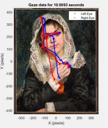
To demonstrate the general strategy for using the TRACKPixx3, we will program a short free viewing task. In this task, participants are given 10 seconds to examine a painting displayed on the screen. We record eye position data and then import it from the buffer, and plot gaze paths for the left and right eyes superimposed over the painting itself. 

In this section we will go step-by-step through creating and running this task. To follow along with the code in MATLAB, download the supplementary materials available in the left-hand menu.  These materials include sample buffer data and a copy of the displayed painting, Renoir’s Lise in a White Shawl. 

Below is the plotted sample data, which shows a characteristic pattern of focusing on facial features. 

Step 1: Adjusting and focusing the camera

This project assumes your TRACKPixx3 is connected to your computer and positioned below your display. For tips on initial device setup, see the TRACKPixx3 user guide.

For each participant, it is typically necessary to adjust the camera position to focus on the participant’s eyes. The face should be well-lit by the infrared lamp. Make sure the TRACKPixx3 is powered on by opening PyPixx and selecting “Wake TRACKPixx.” The live camera feed is available in PyPixx > Demo > TRACKPixx.

You can use this feed to make adjustments to the camera and lamp position. The goal is to center the eyes in the feed and ensure the face is evenly lit. 

In almost all cases, it is best to set the LED illuminator intensity to the maximum setting of 8. The illuminator intensity can be changed by clicking on the Settings icon on the TRACKPixx demo screen.

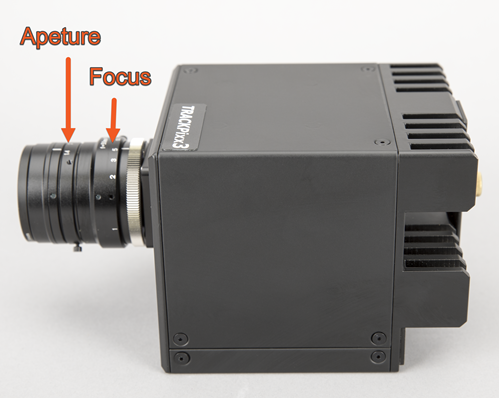
Using the maximum illuminator intensity gives us the most flexibility in terms of how much we can adjust the lens aperture. The aperture is an iris that controls the amount of light let into the camera, and it can be adjusted by rotating the outer ring on the camera lens (see below).

The smaller the camera aperture is, the larger the depth of field, meaning a wider range of depths can be brought into focus at the same time. Ideally, we want a bright light source and a small camera aperture in order to achieve the largest possible depth of field. This ensures we can still track well even if the participant’s head is slightly tilted in the chinrest, or is otherwise not parallel with the camera itself.   

After adjusting the camera aperture, adjust the focus by rotating the large inner ring on the camera lens. The goal here is a crisp image of the eyes, and in particular a clearly defined corneal reflection.

Step 2: Calibration

PyPixx provides a built-in, two-step calibration procedure. Calibration is saved on the device until it is cleared, or your DATAPixx3 is turned off.

While it is possible to perform a calibration directly in MATLAB and Python, this requires a few additional coding steps. For simplicity, in this tutorial we will use PyPixx’s built-in calibration procedure before switching to MATLAB for our viewing task.

Calibration is simple. First, click on the “Pupil Size Calibration” button in PyPixx > Demos > TRACKPixx, and follow the instructions on the screen. Next, click on “Gaze Calibration” and follow the steps on the screen. When both calibrations have been successfully performed, you will see green lights beside the calibration buttons. You can confirm calibration results by launching the Gaze Follower utility and asking participants to follow the mouse with their eyes.

Now that we are calibrated, we can minimize PyPixx and get started with our task.

If your participant moves substantially, or you change participants, you will need to recalibrate to ensure the best tracking. When in doubt–recalibrate!

Step 3. Setting up a schedule

In MATLAB, we need to connect to our DATAPixx device in order to send commands to our hardware. The first command is therefore “Open”.

We follow this with a series of commands to wake up the eye tracker, and set up a TRACKPixx3 schedule. Our schedule controls how the eye tracker records information in the DATAPixx3’s memory. 

We don’t want to start recording just yet. The “SetupTPxSchedule” simply initializes a schedule and then waits for a separate command to start. We will use the default schedule setup for now, so no arguments are needed.

We end this block with a register write, which commits our changes to the device. For more details on the register system, see our guide to registers and schedules.

%Connect to TRACKPixx3
Datapixx('Open');
Datapixx('SetTPxAwake');
Datapixx('SetupTPxSchedule');
Datapixx('RegWr');

Step 4. Showing our target and collecting data

Next, we will open an onscreen window and draw our image. We want to give our participants a bit of warning that the painting will be displayed, so we implement a simple countdown before the painting appears.

We want to start our tracking as soon as our painting is flipped to the screen. Just before we flip our image, we call “StartTPxSchedule”, which will trigger recording on the next register write, and “SetMarker”, which creates a timestamp on the next register write.

Then, we use “RegWrVideoSync” followed by our screen flip. The register write will implement our start and our marker on the next frame of the video signal, which is the same frame where our stimulus appears.

%open window
screenID = 2;                                      
[windowPtr, rect]=Screen('OpenWindow', screenID, [0,0,0]);

%load our image. The jpg is included in the supplementary file download. We will create a rect that
%defines where the painting will appear on the screen
im = imread('Renoir_Lise.jpg');
imTexture = Screen('MakeTexture', windowPtr, im); 
imDimensions = [723.2 862.4];
imRect = [rect(3)/2 - imDimensions(1)/2,...
          rect(4)/2 - imDimensions(2)/2,...
          rect(3)/2 + imDimensions(1)/2,...
          rect(4)/2 + imDimensions(2)/2];         

%show countdown
for k=1:3
    DrawFormattedText(windowPtr, int2str(k), 'center', 700, 255);
    Screen('Flip', windowPtr);
    WaitSecs(1);
end

%draw our image in Screen coordinates (0,0 is top left corner)
Screen('DrawTexture', windowPtr, imTexture, [], imRect);

%start logging eye data on the next vertical sync pulse: the start of the frame with our image  
Datapixx('StartTPxSchedule');
Datapixx('SetMarker');
Datapixx('RegWrVideoSync');

%flip our image to the screen
Screen('Flip', windowPtr);

After a 10 second wait, we will stop recording and pass this command to the device register immediately. We also want to read the contents of the device register set (including retrieving the current time, as well as our timestamp from when we started), so we will do a register write-read. Finally, we close the display.

%wait
WaitSecs(10);

%stop immediately and get some timestamps
Datapixx('StopTPxSchedule');
Datapixx('RegWrRd');
startTime = Datapixx('GetMarker');
endTime = Datapixx('GetTime');
viewingTime = endTime - startTime;

%close our display
Screen('Closeall');

Step 5. Importing data and shutting off TRACKPixx3

We now have 10 seconds of eye tracking data saved in a buffer in our DATAPixx3. Because we performed a register write-read at the end of our tracking period, the local register has the most up-to-date status of our buffer.

We can access this status with “GetTPxStatus,” which returns a structure that includes the variable “newBufferFrames,” which indicates how many new frames of data we have collected since we started our schedule.

“ReadTPxData” imports the requested number of frames to the local register. Since we want everything in the buffer, we pass this function the value we read from newBufferFrames.

Each imported frame has 20 columns of data. We’ve covered the contents of each buffer in a previous section.

We convert this data array into a MATLAB table, with variable labels. Then we save our data as both a .mat file, and as a .csv using MATLAB’s ‘writetable’ function.

As a last step, we turn off the TRACKPixx3 lamp and then close our connection with VPixx hardware. 

%retrieve state of our TPx buffer and read new contents
status = Datapixx('GetTPxStatus');
toRead = status.newBufferFrames;
[bufferData, ~, ~] = Datapixx('ReadTPxData', toRead);

%save eye data from trial as a table in the trial structure
TPxData = array2table(bufferData, 'VariableNames', {'TimeTag',...
                                                    'LeftEyeX',...
                                                    'LeftEyeY',...
                                                    'LeftPupilDiameter',...
                                                    'RightEyeX',...
                                                    'RightEyeY',...
                                                    'RightPupilDiameter',...
                                                    'DigitalIn',...
                                                    'LeftBlink',...
                                                    'RightBlink',...
                                                    'DigitalOut',...
                                                    'LeftEyeFixationFlag',...
                                                    'RightEyeFixationFlag',...
                                                    'LeftEyeSaccadeFlag',...
                                                    'RightEyeSaccadeFlag',...
                                                    'MessageCode',...
                                                    'LeftEyeRawX',...
                                                    'LeftEyeRawY',... 
                                                    'RightEyeRawX',...
                                                    'RightEyeRawY'});
%save as both a .mat and .csv file
save('TPxData.mat', 'TPxData');
writetable(TPxData, 'TPxData.csv');

%turn off tracker and disconnect
Datapixx('SetTPxSleep');
Datapixx('RegWr');
Datapixx('Close');

Almost all Datapixx functions require a register write in order to be implemented on your VPixx device. “Open,” “Close,” and “ReadTPxBuffer” are special cases where the command is immediately passed to the device, and no register write is needed.

Step 6. Plotting gaze path

As a last step, we will load our saved data (or sample data) and plot it as an overlay on our painting. 

The trickiest part of this step is adding our image to the figure. Our painting’s location and dimensions are defined in our “imRect” variable, which uses Psychtoolbox Screen coordinates. That is, it treats x =0 and y=0 as the top left corner of the display. In contrast, our camera space and gaze data use a Cartesian coordinate system, where (0,0) is the center of the display. So, if we were to plot the painting and gaze path as is, they won’t line up properly in our figure.

We need to add an offset to imRect so it is plotted in the same coordinate system as our gaze data. There is an existing Datapixx function called “ConvertCoordSysToCartesian” which will do this for us. It assumes a 1920 x 1080 display and provides default offsets for this screen size.

Next, the easy part: plotting left and right eye data from our saved data table, and adding some labels to our graph. 

MATLAB’s “image” plot tool inverts the y axis automatically (so it runs positive -> negative). As a last step, we invert the y axis to reverse the effects of this tool. Now we have a lovely overlay of our gaze path!

%load our saved data
load('TPxData.mat');
%load('TPxSampleData.mat');

%plot image behind, centered on an origin of 0,0 in middle of the screen, which is VPixx eye
%tracking coordinates
figure('Position', [100, 200, 420, 500]);
plotRect(1:2) = Datapixx('ConvertCoordSysToCartesian', imRect(1:2));
plotRect(3:4) = Datapixx('ConvertCoordSysToCartesian', imRect(3:4));
image([plotRect(1), plotRect(3)],[plotRect(2), plotRect(4)], im);
hold on

%plot our data
plot(TPxData.LeftEyeX(:), TPxData.LeftEyeY(:), '.b');
plot(TPxData.RightEyeX(:), TPxData.RightEyeY(:), '.r');

%add some labels
legend('Left Eye', 'Right Eye');
xlabel('X (pixels)');
ylabel('Y (pixels)');
titlestr =['Gaze data for ' num2str(round(viewingTime,4)) ' seconds'];
title(titlestr);

%the 'image' function flips the y axis; now that all data is plotted we'll flip it back
ax = gca;
ax.YDir='normal';

And the final product:

Still have questions about the TRACKPixx3, or features you’d like to see? Contact our support team at support@vpixx.com. Happy tracking! 

Notes

The painting used in this project is Pierre-Auguste Renoir’s “Lise in a White Shawl.” This image is considered public domain and can be freely reproduced. Image file courtesy of Wikimedia Commons and the Dallas Museum of Art.