Rapid Invisible Frequency Tagging (RIFT) using the PROPixx 1440 Hz mode

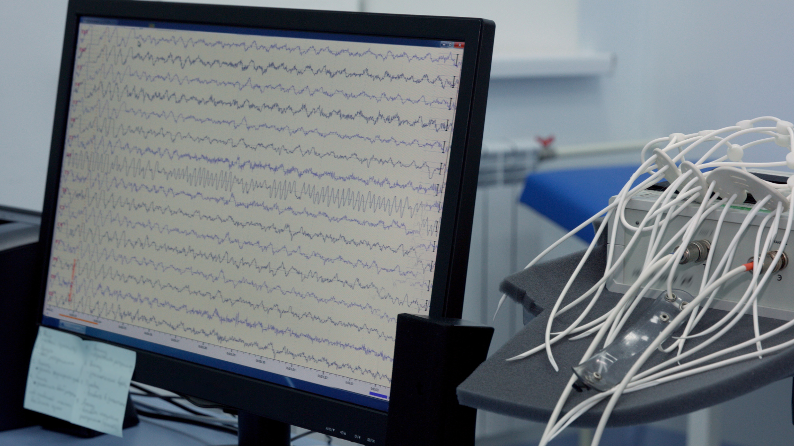
Frequency tagging uses flickering stimuli to evoke signals at the same frequencies in the brain. These signals, called steady state visually evoked potentials (SSVEPs) in EEG and steady state visually evoked fields (SSVEFs) in MEG/OPM, can shed light on visual and cognitive processes. For instance, the relative amplitude of SSVEPS can reflect processes like attention, and the progression of the signal across brain regions demonstrates the pathway of visual information processing.

*EEG traces can be analyzed to reveal frequencies evoked by the stimulus display*

Traditional frequency tagging paradigms use visibly flickering stimuli (e.g., < 60 Hz). Low-frequency tagging has some disadvantages:

they can irritate and make participants uncomfortable
they can obscure other low-frequency signals of interest
they can make it difficult to measure specific kinds of cognitive and perceptual processes (e.g., covert attention)

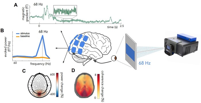
Researchers at the University of Birmingham have demonstrated that a smoothly modulated or sinusoidal flicker >60 Hz can reliably evoke SSVEMs while remaining invisible to the participant. This method, called Rapid Invisible Frequency Tagging (RIFT), opens up many new avenues for research; since its inception, it has been used to study brain-computer interfaces, language perception, attention and more.

A key advantage of RIFT is that experimental paradigms can be ‘hidden’ in naturalistic tasks without alerting the participant. This makes them ideal for more extended studies or testing special populations like children.

For an excellent review of RIFT from a research perspective, we recommend this article:

Methodologically, RIFT can only be achieved using a high-speed display. The display must update fast enough to generate a smoothly modulated flicker that maintains a target frequency > 60 Hz.

This is where the PROPixx comes in. The QUAD12X mode on the projector operates at 1440 frames per second in greyscale, allowing for high-speed frame transitions with the temporal resolution required to support RIFT applications. Indeed, to our knowledge, the PROPixx remains the only research-grade display solution used in RIFT paradigms where complex visual stimuli are needed.

The rest of this guide reviews QUAD12X mode and uses it to present a high-speed modulating stimulus with a custom frequency set by the user. We will measure the resultant display luminance changes using a photodiode to show the projector output is modulating smoothly, and we will discuss the relationship between synchronization signals from VPixx hardware and display timing.

QUAD12X: 1440 Hz in greyscale

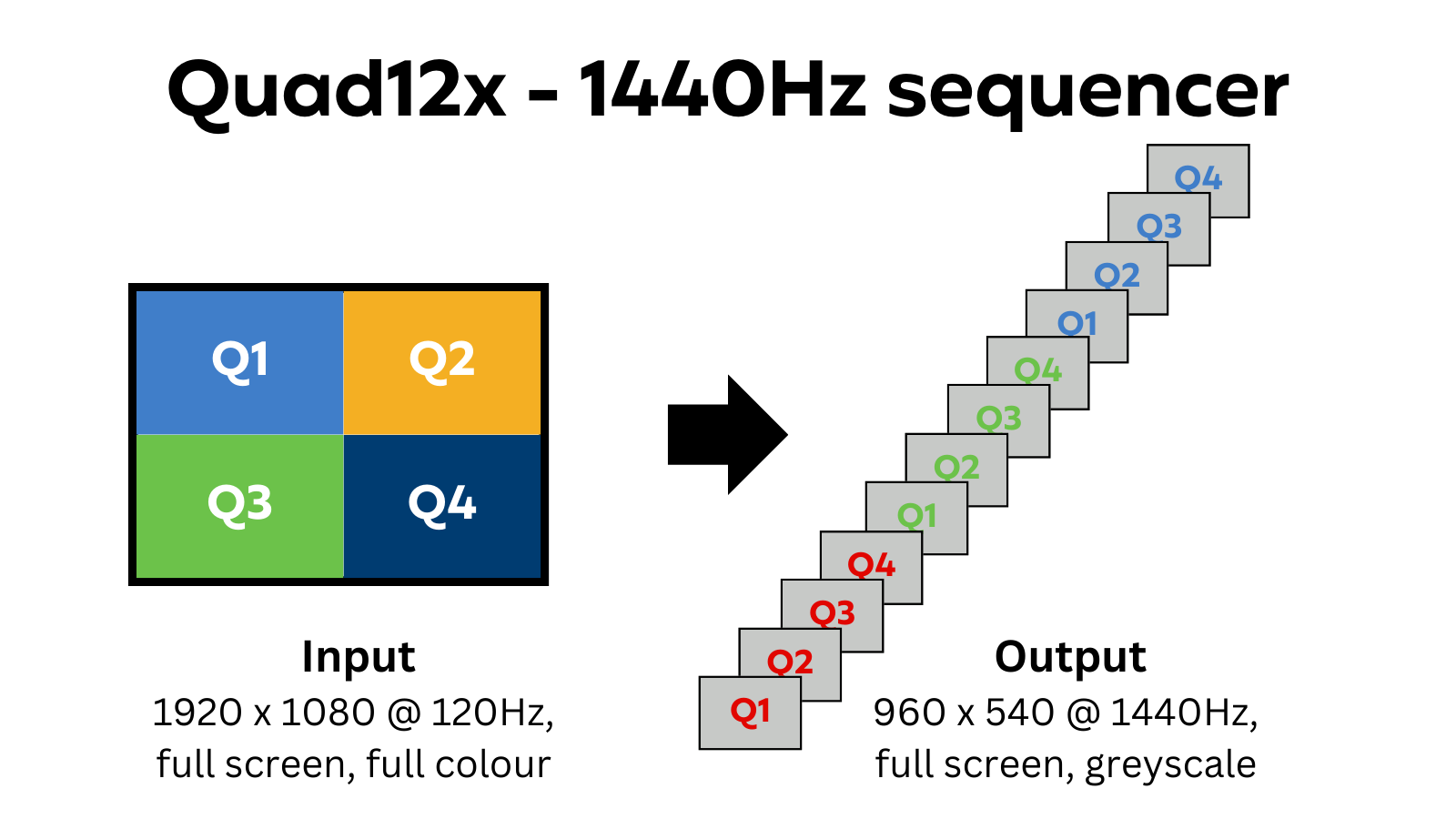
In QUAD12X mode, the PROPixx receives full HD resolution video (1920 x 1080) at 120 Hz from your PC. It then ‘breaks down’ each frame of this video into 12 distinct subframes. It shows each subframe in a sequence; each subframe is shown full screen, greyscale. This produces a final display refresh rate of 1440 Hz (120 x 12).

The order in which a composite 120 Hz image is broken down is as follows:

The image is subdivided into four ‘quadrants’
Each quadrant is further divided into red, green and blue colour channels, and interpreted as 8 bit greyscale
The subframes are shown in the following order: Q1R, Q2R, Q3R, Q4R, Q1G …. Q4B

QUAD12x sequencer

For more details on QUAD12X, including links to other demos showing its implementation, see Quad12x: 1440Hz greyscale, half resolution.

Using QUAD12X to generate a sinusoidal mask

Following the example in Seijdel et al. (2023), we will present a static image in the center of the display, with a 68 Hz sinusoidal mask applied overtop, for 10 seconds. The code can easily be modified for different target frequencies.

Tiling the stimulus into quadrants

First, we must configure our ‘composite’ 120 Hz stimulus to format the 1440 Hz output correctly. We will use this as our stimulus:

As a first step, we must tile this stimulus to appear in the center of all four quadrants in our composite image. This will ensure it appears in the center of the 1440 Hz display on each subframe. Remember, the images in each quadrant will be shown full-screen, twice as large, in the final output.

A simple helper function loads and tiles the 960 x 540 image and background. Click on the tab below to expand the section and view the code.

createTiledTexture

MATLAB

function tiledTexture = createTiledTexture(imagePath)
    % CREATE TILED TEXTURE
    % This function loads a 960x540 PNG image and tiles it 2x2
    % to generate a 1920x1080 image texture.
    %
    % INPUT:
    %   imagePath - Path to the 960x540 PNG image file.
    %
    % OUTPUT:
    %   tiledTexture - 1920x1080 texture formed by tiling the image.

    % Load the PNG image
    img = imread(imagePath);

    % Check if the image is 960x540, if not, show an error
    [height, width, ~] = size(img);
    if (height ~= 540 || width ~= 960)
        error('Input image must be 960x540 in size.');
    end

    % Tile the image 2x2
    tiledTexture = repmat(img, 2, 2);
end

Because our stimulus is already in greyscale and static, this is all we need to do to format it. If this were a dynamic or colour image, we would need to generate a more complex image that ‘zeros’ the colour channels not associated with the target subframes. For instance, an image shown exclusively on the first four subframes (red colour channel) should not have any blue or green colour data. Composite images with data in more than one colour channel will be split into the relevant subframes:

Sequencers (4).png — *Blue and red channels*

Generating the mask transparencies for sinusoidal output

Now, let’s consider our mask. We need to identify each subframe's transparency level to generate a smooth oscillation between transparent and opaque. This is a slowed-down version of what we want the result to look like:

*Mask with oscillating transparency from fully transparent → opaque*

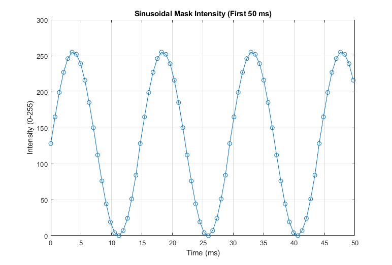
First, we generate a sinusoid of transparency values from 0 - 255 with our target frequency of 68 Hz using a helper function. Click on the expand tab to view the function code.

generateTransparencyValues

MATLAB

function transparency = generateTransparencyValues(stimFreq, duration)
    % GENERATE TRANSPARENCY ARRAY
    % Generates a sine-wave-based transparency array for a 1440 
    % Hz stimulus.
    %
    % INPUTS:
    %   stimFreq  - Sinusoidal frequency in Hz (e.g., 68)
    %   duration  - Total duration in seconds (e.g., 10)
    %
    % OUTPUTS:
    %   transparency - Array of transparency values (0-255)
    %   t            - Corresponding time vector in seconds

    % Fixed frame rate
    frameRate = 1440;  

    % Calculate the number of frames per cycle
    nFrames = frameRate / stimFreq;

    % Generate time vector for one full cycle
    tCycle = linspace(0, (nFrames - 1) / frameRate, nFrames);

    % Compute transparency values using a sine wave (0-255 range)
    transparencyCycle = 127.5 + 127.5 * sin(2 * pi * stimFreq * tCycle);

    % Round to nearest integer for valid 8-bit transparency values
    transparencyCycle = round(transparencyCycle);

    % Determine the total number of cycles for the given duration
    % We add a small buffer to the duration in case we go slightly over time over time in our presentation loop
    numCycles = round((duration + 5) * stimFreq);

    % Repeat the cycle to fill the full duration
    transparency = repmat(transparencyCycle, 1, numCycles);

end

Here’s what the first 50 ms of transparency samples look like, plotted:

*Intensities for a 68 Hz signal divided into 1440 frames/second*

Formatting mask to ensure correct subframe assignment

The mask is a circle that covers the image and oscillates its transparency 0-255. We know the transparency value on each subframe, the final desired position of the mask (center of the frame) and the size (diameter = width of the stimulus image). To build our composite 120 Hz image we need to draw 12 of these masks in a single framebuffer, along with our tiled background, then pass everything to the display.

When drawing each of our 12 masks, we need to ensure:

The colour channel corresponds to the correct target subframe
The blend mode is set correctly (see the section below)
The position of the mask is offset to reflect its quadrant

The helper function drawCircularMask does all of these steps for us automatically. We need to pass it the mask properties and subframe number, and it will do the rest.

drawCircularMask

MATLAB

function drawCircularMask(windowPtr, transparency, subframe, x, y, diameter)
    % DRAW CIRCULAR MASK WITH COLOR AND TRANSPARENCY
    % This function draws a circular mask at a specified position, 
    % with color and transparency based on the subframe index.
    %
    % INPUTS:
    %   windowPtr    - Pointer to the Psychtoolbox window
    %   transparency - Alpha transparency value (0 = fully transparent, 255 = fully opaque)
    %   subframe     - Determines position offset and color (1-12)
    %   x, y         - Base position of the circle (center coordinates)
    %   diameter     - Diameter of the circle in pixels
    %
    % OUTPUT:
    %   A colored circle with the specified transparency drawn in the window

    % Determine color and blend function based on subframe using mod
    colorIndex = mod(subframe - 1, 12); % Normalize subframe to range [0, 11]
    
    if colorIndex < 4
        color = [255, 0, 0, transparency];  % Red component
        blendColor = [1, 0, 0, 0];
    elseif colorIndex < 8
        color = [0, 255, 0, transparency];  % Green component
        blendColor = [0, 1, 0, 0];
    else
        color = [0, 0, 255, transparency];  % Blue component
        blendColor = [0, 0, 1, 0];
    end
    
    % Apply blend function
    Screen('BlendFunction', windowPtr, GL_SRC_ALPHA, GL_ONE_MINUS_SRC_ALPHA, blendColor);
    
    % Compute the radius from the given diameter
    radius = (diameter / 2);

    % Determine position offset based on subframe index
    switch mod(subframe - 1, 4) + 1
        case 1
            offset = [-960/2, -540/2];  % Top-left quadrant
        case 2
            offset = [960/2, -540/2];   % Top-right quadrant
        case 3
            offset = [-960/2, 540/2];   % Bottom-left quadrant
        case 4
            offset = [960/2, 540/2];    % Bottom-right quadrant
    end

    % Apply offset to the base position
    position = [x, y] + offset;

    % Define the bounding box for the circular mask
    rect = [position(1) - radius, position(2) - radius, ...
            position(1) + radius, position(2) + radius];

    % Draw the circular mask with the computed color and transparency
    Screen('FillOval', windowPtr, color, rect);

    % Reset blend function to default after drawing
    Screen('BlendFunction', windowPtr, GL_SRC_ALPHA, GL_ONE_MINUS_SRC_ALPHA, [1, 1, 1, 1]);
end

On blending functions and overlapping stimuli

In many cases, when building the composite image for our display, layers in the image will overlap one another. In this case, the software has to decide how to combine the layers; this process is called blending. Most software will, by default, treat opaque layers as obscuring the layers beneath them. If a layer is semi-transparent, the software typically computes a weighted average of this layer and the one below it (alpha blending). An alternative is additive blending, where colour channel data is independent and sums in the final display.

Sequencers (9).png — *Types of blending*

In QUAD12X mode, we need to perform alpha blending within a colour channel and additive blending across channels to preserve all of the grayscale data in different subframes of the final 1440 Hz display.

Fortunately, this can easily be done in MATLAB with the Screen('BlendFunction') command from Psychtoolbox:

MATLAB

#Alpha blend red channel, do not alter other channel data
Screen('BlendFunction', windowPtr, GL_SRC_ALPHA, GL_ONE_MINUS_SRC_ALPHA, [1 0 0 0]);

This results in alpha blending the specified colour channel in the list [r, g, b, alpha] while leaving other channels (set to 0) unaffected.

To implement this in Python is a bit more challenging. Presently, PsychoPy windows do not support channel-specific blending options, so we must invoke a custom shader that does what we described above.

PY

code coming soon!

Putting it all together

So far we have identified several discrete steps for generating a composite image in our RIFT display. They are:

Tile our static, greyscale 960 x 540 image into four quadrants
Generate a list of transparencies for our 68 Hz mask
Generate 12 masks for our composite image using our transparency list and our helper function

As a reminder, we want our final display to look like this (but much faster):

Below is the entire MATLAB and Python code to achieve this output. You can download the stimulus image here: [download]. Make sure it is in the same folder as your test script.

RIFT Demo - MATLAB

MATLAB

//%%%%MAIN SCRIPT
%Set some important variables
imagePath = 'logo_960x540.png';
tiledTexture = createTiledTexture(imagePath);
AM
stimFreq = 68; % Hz
duration = 20; % seconds
transparency = generateTransparencyValues(stimFreq, duration); % list of transparency values
maskDiameter = 600; % covers the whole logo

% Initialize VPixx Hardware
isConnected = Datapixx('isReady');
if ~isConnected
    Datapixx('Open');
end
Datapixx('SetPropixxDlpSequenceProgram', 5);        %Set Propixx to 1440Hz refresh (also known as Quad12x)
Datapixx('RegWrRd');   

% Initialize Psychtoolbox
screenID = max(Screen('screens'));
windowPtr = Screen('OpenWindow', screenID, [255,255,255]); % Open fullscreen window with white background
Screen('BlendFunction', windowPtr, GL_SRC_ALPHA, GL_ONE_MINUS_SRC_ALPHA);  % Set blend mode
stimulus = Screen('MakeTexture', windowPtr, tiledTexture);  % Create texture from image

% Get initial time & transparency index
Datapixx('RegWrRd');
t1 = Datapixx('GetTime');
t2 = t1;
index = 1;

while (t2 - t1) < duration

    % Display the tiled image
    Screen('DrawTexture', windowPtr, stimulus);  

    % Loop through 12 iterations of masks
    for subframe = 1:12
        drawCircularMask(windowPtr, transparency(index), subframe, 0, 0, maskDiameter);
        index = index+1;       

    end
    Screen('Flip', windowPtr);
    Datapixx('RegWrRd');
    t2 = Datapixx('GetTime');
end

% Close down after the loop
Screen('CloseAll');
Datapixx('SetPropixxDlpSequenceProgram', 0);        
Datapixx('RegWrRd');  
Datapixx('Close');


%% HELPER FUNCTIONS

function tiledTexture = createTiledTexture(imagePath)
    % CREATE TILED TEXTURE
    % This function loads a 960x540 PNG image and tiles it 2x2
    % to generate a 1920x1080 image texture.
    %
    % INPUT:
    %   imagePath - Path to the 960x540 PNG image file.
    %
    % OUTPUT:
    %   tiledTexture - 1920x1080 texture formed by tiling the image.

    % Load the PNG image
    img = imread(imagePath);

    % Check if the image is 960x540, if not, show an error
    [height, width, ~] = size(img);
    if (height ~= 540 || width ~= 960)
        error('Input image must be 960x540 in size.');
    end

    % Tile the image 2x2
    tiledTexture = repmat(img, 2, 2);
end


function transparency = generateTransparencyValues(stimFreq, duration)
    % GENERATE TRANSPARENCY ARRAY
    % Generates a sine-wave-based transparency array for a 1440 
    % Hz stimulus.
    %
    % INPUTS:
    %   stimFreq  - Sinusoidal frequency in Hz (e.g., 68)
    %   duration  - Total duration in seconds (e.g., 10)
    %
    % OUTPUTS:
    %   transparency - Array of transparency values (0-255)
   
    % Fixed frame rate
    frameRate = 1440;  

    % Calculate the number of frames per cycle
    nFrames = frameRate / stimFreq;

    % Generate time vector for one full cycle
    tCycle = linspace(0, (nFrames - 1) / frameRate, nFrames);

    % Compute transparency values using a sine wave (0-255 range)
    transparencyCycle = 127.5 + 127.5 * sin(2 * pi * stimFreq * tCycle);

    % Round to nearest integer for valid 8-bit transparency values
    transparencyCycle = round(transparencyCycle);

    % Determine the total number of cycles for the given duration
    % We add a small buffer to the duration in case we go slightly over time in our presentation loop
    numCycles = round((duration + 5) * stimFreq);

    % Repeat the cycle to fill the full duration
    transparency = repmat(transparencyCycle, 1, numCycles);

end

function drawCircularMask(windowPtr, transparency, subframe, x, y, diameter)
    % DRAW CIRCULAR MASK WITH COLOR AND TRANSPARENCY
    % This function draws a circular mask at a specified position, 
    % with color and transparency based on the subframe index.
    %
    % INPUTS:
    %   windowPtr    - Pointer to the Psychtoolbox window
    %   transparency - Alpha transparency value (0 = fully transparent, 255 = fully opaque)
    %   subframe     - Determines position offset and color (1-12)
    %   x, y         - Base position of the circle (center coordinates)
    %   diameter     - Diameter of the circle in pixels
    %
    % OUTPUT:
    %   A colored circle with the specified transparency drawn in the window

    % Determine color and blend function based on subframe using mod
    colorIndex = mod(subframe - 1, 12); % Normalize subframe to range [0, 11]
    
    if colorIndex < 4
        color = [255, 0, 0, transparency];  % Red component
        blendColor = [1, 0, 0, 0];
    elseif colorIndex < 8
        color = [0, 255, 0, transparency];  % Green component
        blendColor = [0, 1, 0, 0];
    else
        color = [0, 0, 255, transparency];  % Blue component
        blendColor = [0, 0, 1, 0];
    end
    
    % Apply blend function
    Screen('BlendFunction', windowPtr, GL_SRC_ALPHA, GL_ONE_MINUS_SRC_ALPHA, blendColor);
    
    % Compute the radius from the given diameter
    radius = (diameter / 2);

    % Determine position offset based on subframe index
    switch mod(subframe - 1, 4) + 1
        case 1
            offset = [-960/2, -540/2];  % Top-left quadrant
        case 2
            offset = [960/2, -540/2];   % Top-right quadrant
        case 3
            offset = [-960/2, 540/2];   % Bottom-left quadrant
        case 4
            offset = [960/2, 540/2];    % Bottom-right quadrant
    end

    % Apply offset to the base position
    position = [x, y] + offset;

    % Define the bounding box for the circular mask
    rect = [position(1) - radius, position(2) - radius, ...
            position(1) + radius, position(2) + radius];

    % Draw the circular mask with the computed color and transparency
    Screen('FillOval', windowPtr, color, rect);

    % Reset blend function to default after drawing
    Screen('BlendFunction', windowPtr, GL_SRC_ALPHA, GL_ONE_MINUS_SRC_ALPHA, [1, 1, 1, 1]);
end

RIFT Demo - Python

CODE

Coming soon!

Is it working?!

The whole point of RIFT is that the oscillation is invisible. If you see a static grey logo on the display, don’t worry! The code is working. Try changing the stimFreq to a lower value, like 5 Hz, to see the oscillation.