Visualizing Gaze Data

The TRACKPixx3 records eye tracking data at a rate of 2000 samples per second. During recording, these data are saved in the DATAPixx3’s onboard memory. Data can then be bulk imported directly into MATLAB or Python as an m x 20 array, where m is the number of samples recorded. 

Details on the contents of the 20 columns, and instructions for recording and importing TRACKPixx3 data, are described in Introduction to Eye Tracking with the TRACKPixx3. In this guide, we walk through some methods for visualizing eye-tracking data in MATLAB.

First, we will talk a bit about formatting tips for easy navigation of your raw data. Next, we will show how to generate the following four figures: raw gaze path, a gaze heat map, and ordered fixations and saccades (based on TRACKPixx3’s automatic flagging system).

Gaze data visualization for a single 15-second free viewing

You do not need any VPixx hardware for this project. There is a download link in the sidebar that provides sample gaze data that you can use to generate visualizations in MATLAB. The code is also provided; we will go through it step-by-step below.

If you prefer to visualize your own collected data, follow the formatting steps in the next section to use in the rest of the project. 

Formatting your data

For the purposes of this project, we will only visualize data from a single recorded trial. The sample data for this project is stored in a .mat file containing a data structure named TrialData: 

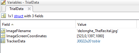
TrialData contains several fields including:

• ImageFileName: a string with the name of our visual stimulus, to use as a plot background. This file should be in your working directory, or somewhere on your path.

• ImageScreenCoordinates: a 1×4 vector with the format [x1 y1 x2 y2], describing where the image was shown on the screen during recording. The coordinates (x1, y1) denote the location of the top left corner of the image, in Psychtoolbox screen coordinates (top left corner of the display is 0,0). The coordinates (x2, y2) are the location of the bottom right corner of the image. 

• TrackerData: a 20-column table of raw data from the TRACKPixx3 

If you’ve followed some of our other TRACKPixx3 demos or projects, you may recognize the table format of our tracker data.  This is not the raw output of the tracker, which is an unlabeled 20-column array.

While formatting eye tracking data as a table is not necessary, it does make the data easier to interpret and work with. Tables allow us to label our columns of data with intuitive names like “RightPupilDiameter” and “LeftEyeFixationFlag.” We can then access specific columns with dot indexing, e.g., myData.LeftEyeFixationFlag . 

Most of our MATLAB demos immediately convert our recorded eye data into a table format. For those using their own recorded data, the function convertToTPxTable included in the supplementary materials can convert an m x 20 MATLAB array into a properly labeled TRACKPixx3 table. 

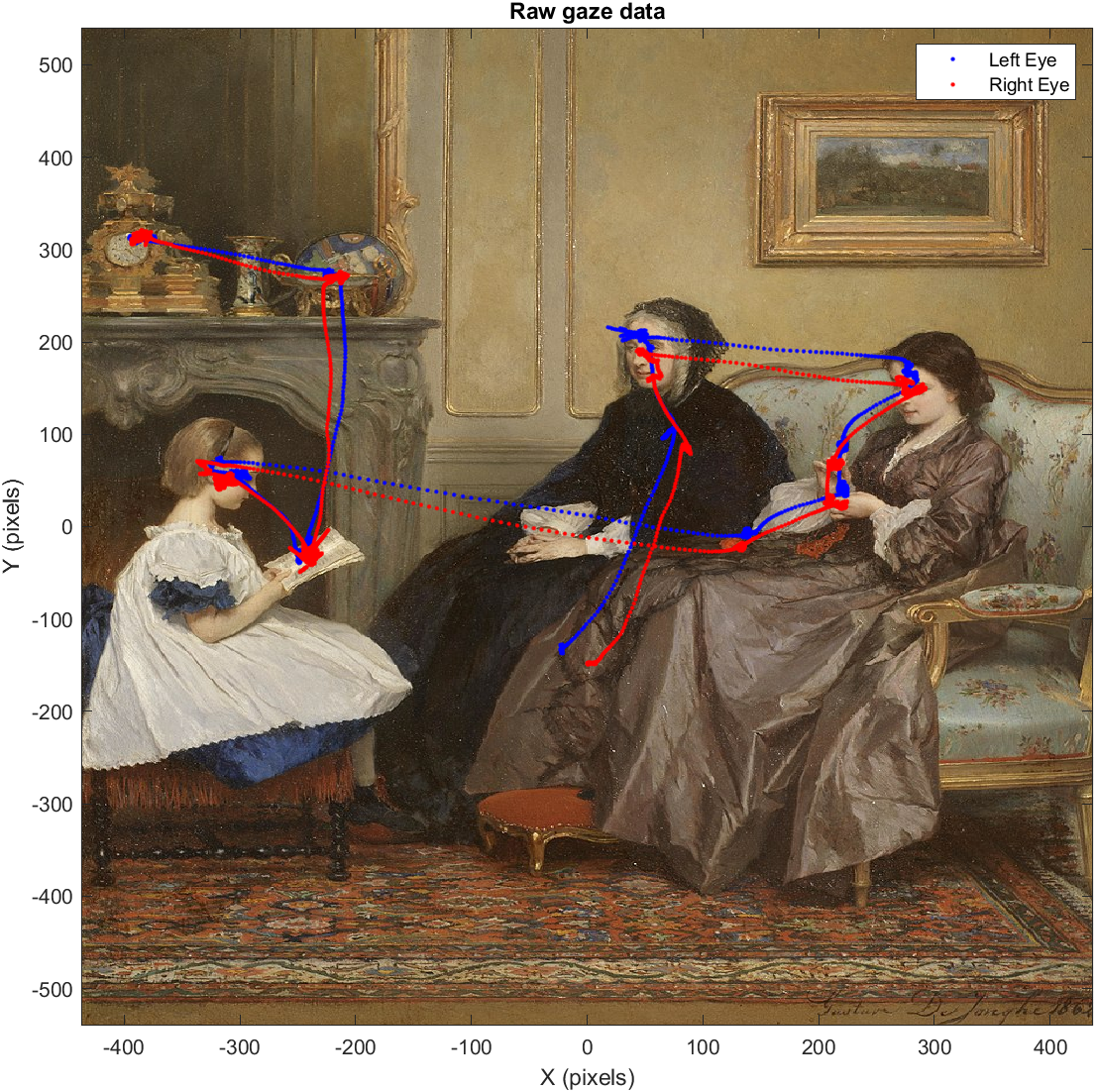
Plotting raw gaze data

The simplest visualization we will cover is simply plotting all of the gaze data we have for the left and right eye. 

To overlay this data over the sample image itself, we must draw the image in our plot. However, our image dimensions are currently in Psychtoolbox screen coordinates, which place (0,0) in the top left corner of the display. Our eye tracker coordinates use a Cartesian coordinate system, with (0,0) in the middle of the display. 

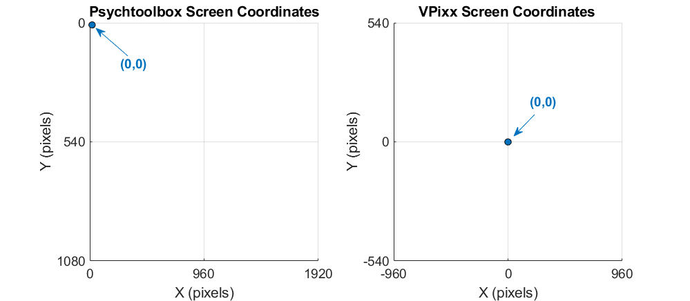
We will keep everything in VPixx screen coordinates. The Datapixx toolbox for MATLAB/Psychtoolbox includes a conversion function that we can use to get our plotting coordinates for our image, which we save as plotRect:

im = imread(TrialData.ImageFilename);
imRect = TrialData.ImageScreenCoordinates;
%convert our image dimensions into Cartesian coordinates, so we can overlay data
plotRect= nan(1,4);
plotRect(1:2) = Datapixx('ConvertCoordSysToCartesian', imRect(1:2));
plotRect(3:4) = Datapixx('ConvertCoordSysToCartesian', imRect(3:4));

Next, let’s create a figure and plot our image using MATLAB’s ‘image’ function. This function automatically flips the Y axis direction; if we do nothing, the image will appear upside-down. We will explicitly set the y axis direction to ‘normal’ to fix this. 

We will set the plot limits to the boundaries of our image, since this is the region we are interested in. We will also add some axis labels and a title.

figure();
%plot our image as a background
image([plotRect(1), plotRect(3)],[plotRect(2), plotRect(4)], im);
hold on
%flip our y axis to correct for the inversion caused by the image function
ax = gca;
ax.YDir='normal';
%set axis limits to the boundaries of our image
xlim(plotRect(1), plotRect(3));
ylim(plotRect(4), plotRect(2));
xlabel('X (pixels)');
ylabel('Y (pixels)');
titlestr ='Raw gaze data';
title(titlestr);

Now we have generated our image background, which can be seen below. As all of our visualizations use this background, we will need to repeat this initial plotting for each of the four figures we will generate in this tutorial. 

To plot our raw gaze data, we will use dot indexing to get all of our x and y data for the left and right eyes. We will plot these in blue and red, respectively, and add a legend in the default position:

%plot left and right eye traces
plot(TrialData.TrackerData.LeftEyeX(:), TrialData.TrackerData.LeftEyeY(:), '.b');
plot(TrialData.TrackerData.RightEyeX(:), TrialData.TrackerData.RightEyeY(:), '.r'); 
%add some labels
legend('Left Eye', 'Right Eye');

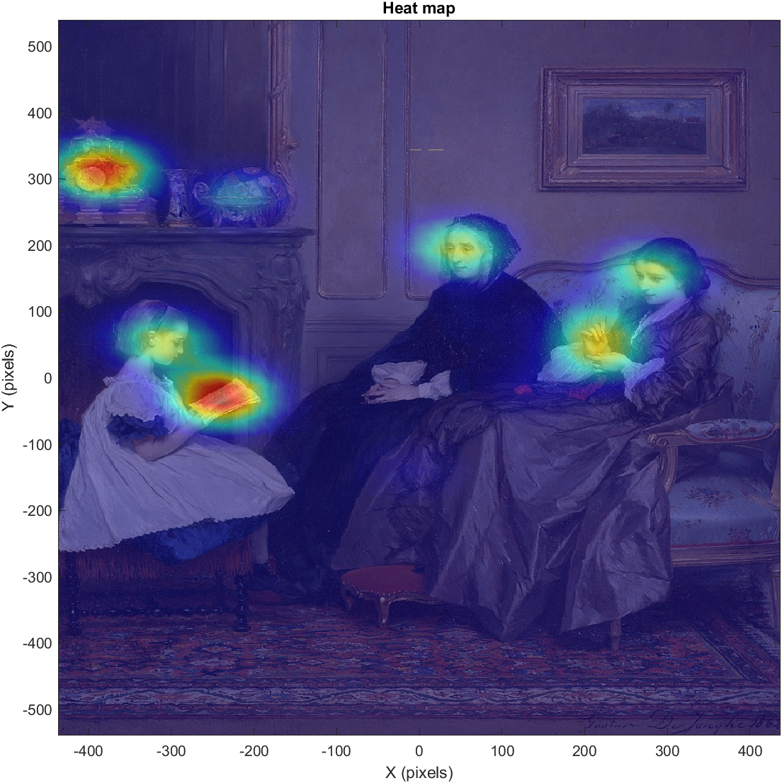
Generating a gaze heat map

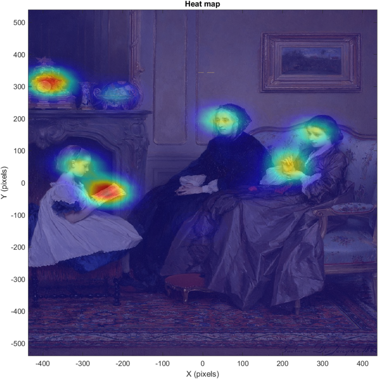
A heat map is a probability map showing the likelihood of any particular point in the image to be looked at, given our raw gaze data. These probability values are based on a kernel density estimation, which takes our gaze data and produces a probability distribution across the image. It is important to remember that heat maps do not show raw data, but a estimated distribution based on raw data.

We will use an existing function for performing our kernel density estimation, gkde2.m, which was authored by Yi Cao at Cranfield University. We pass this function our average x and average y gaze data, and it returns a structure with our probability function.  You’ll notice two artificial data points have been added to our average x and y data. These are the corners of our plotted image in VPixx screen coordinates. Adding these points to our data ensures that the resulting density function covers the entire region of our displayed image, even if our participants didn’t look near the edges of the image during recording. If we leave these points out, our resulting map will only reach the bounds of the space defined by our data, plus a small margin. 

%average left and right eye data
xavg = mean([TrialData.TrackerData.LeftEyeX, TrialData.TrackerData.RightEyeX], 2, 'omitnan');
yavg = mean([TrialData.TrackerData.LeftEyeY, TrialData.TrackerData.RightEyeY], 2, 'omitnan');
%Submit gaze data to a bivariate kernel density function to get a probability distribution. We add
%plotRect to to the data to ensure the function scales to the full image size.
avgData = [xavg, yavg; plotRect(1:2); plotRect(3:4)];
p = gkde2(avgData);

If we plot the results of p, we get a probability distribution, where x and y are screen coordinates and z indicates likelihood. If we collapse the z axis we are left with the colour patches indicating relative elevation. This can be overlaid on our image to create a heat map.

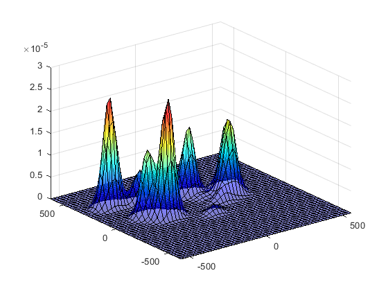
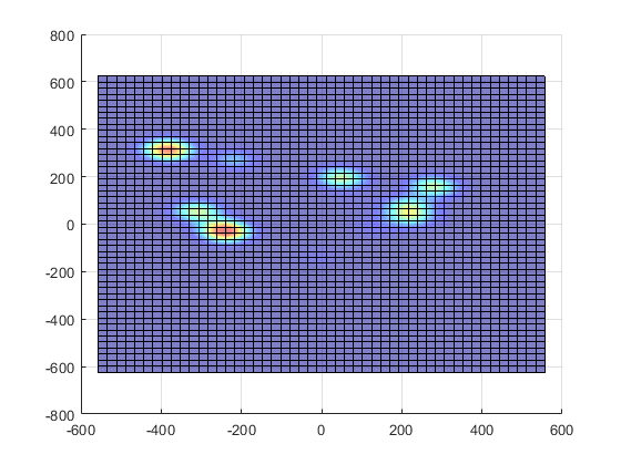
Probability density function for our raw gaze data, in 3D (left) and with the z-axis collapsed (right)

You can tweak the plot characteristics to your liking. The following code shows how to generate the heat map featured below. This code snippet assumes you have already scaled your background image, which we covered in the previous section.

%plot our image as a background
figure();
image([plotRect(1), plotRect(3)],[plotRect(2), plotRect(4)], im);
hold on
%flip our y axis to correct for the inversion caused by the image function
ax = gca;
ax.YDir='normal';
%set axis limits to the boundaries of our image
xlim([plotRect(1), plotRect(3)]);
ylim([plotRect(4), plotRect(2)]);
xlabel('X (pixels)');
ylabel('Y (pixels)');
titlestr ='Heat map';
title(titlestr);
%plot the distribution
surf(p.x,p.y,p.pdf...
    'FaceAlpha',0.5,...
    'AlphaDataMapping','scaled',...
    'AlphaData',p.pdf...
    'FaceColor','interp',...
    'EdgeAlpha',0);
colormap(jet)
%return to 2d view 
view(2)

And the result:

Plotting fixation data

Fixations refer to moments in the trial where the participant is foveating a specific part of the image, and their eyes are not moving. Fixations are automatically flagged by the TRACKPixx3. The default setting, which we use here, is that fixations occur when the eye is moving less than 2500 pixels/second, for more than 25 frames. This setting can be changed in either PyPixx or MATLAB. 

In this section we will cover how to perform some preliminary analysis on fixations, and how to visualize this information. We will start by examining the finished product. There is a lot of information in this visualization, and we will describe all of it before showing how the plot is generated:

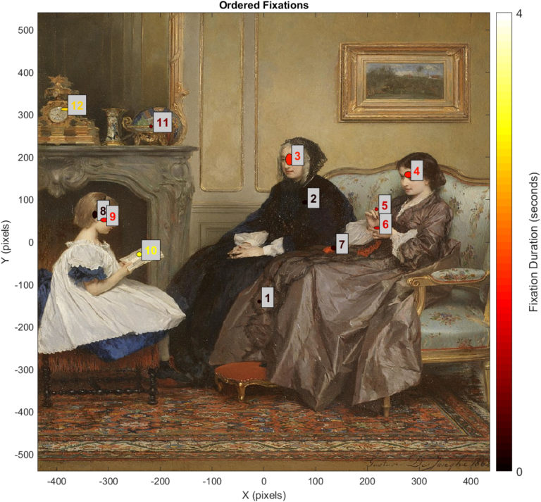
In this plot, fixations have been denoted with a labelled ellipse. 

• The (x, y) coordinates of the center of the ellipse correspond to the average gaze location across the entire fixation. This is based on averaged left and right eye data.

  • The label indicates the temporal order of the fixation 

  • The horizontal axis of the ellipse is +/- 1 standard deviation of the average x location

  • The vertical axis of the ellipse is +/- 1 standard deviation of the average y location

  • The colour of the ellipse and label denote duration. Colour mapping is scaled to the maximum fixation duration observed in the trial

We will also save this data in a summary table, which we will add to our TrialData structure as a new field. 

As a first step, we will go into TrackerData and get our fixation flags. There is a separate column for the left and right eye, and the flags have a value of either 0 (not fixating) or 1 (fixating).

To get a single binocular fixation, we will take the maximum of left and right eye flags. Realistically, a normally-sighted person fixates with both eyes. In practice, a 2 kHz tracker is fast enough to catch jitter between the eyes at fixation onset/offset. By taking the maximum of the two flags, we count even one flag being raised as part of a fixation.

After developing a single list of binocular fixations, we will find flag onsets and offsets and create lists of both.

%let's combine right and left eye flags, by taking the max of the two columns
fixAvg=max([TrialData.TrackerData.LeftEyeFixationFlag, TrialData.TrackerData.RightEyeFixationFlag],[], 2);
%get our fixation starts and stops
fixationStart = find((diff(fixAvg)==1)); 
fixationStop = find((diff(fixAvg)==-1));
%if our participant started with a fixation, let's catch that and add a start on frame 1
if fixationStart(1) > fixationStop(1)
    fixationStart=[1; fixationStart];
end 
%if our participant ended on a fixation, let's catch that and add an end on number of frames
if fixationStop(end) < fixationStart(end)
    fixationStop=[fixationStop; size(fixAvg,1)];
end 

Event flags need to collect a few frames for analysis before raising or lowering. As a result, they lag behind true event onset and offset. With the default settings, the fixation flag raises 15 ms after fixation onset, and lowers 16 ms after it ends. For this project we will simply accept this offset, as it is very small. Researchers interested in adjusting flags to account for raising/lowering time should consult our SaccadeToTarget demo, which includes steps for visualizing kinematics and true fixation/saccade onsets.

Next, we’ll create a table to store our fixation data. For each fixation event in our list, we will loop through our dataset to get the left and right gaze data for the duration of the event. We will calculate mean x and y position, as well as the standard deviation of x and y positions. We will also calculate the duration of the fixation in seconds.

Finally, we store this data in a new table in TrialData, called Fixations.

%create a new table with our fixation data
TrialData.Fixations = table();
for k=1:numel(fixationStart)
    %get average gaze location of both eyes during fixation, and the std of this location
    x = mean([TrialData.TrackerData.LeftEyeX(fixationStart(k):fixationStop(k)), ...
              TrialData.TrackerData.RightEyeX(fixationStart(k):fixationStop(k))],2);
    y = mean([TrialData.TrackerData.LeftEyeY(fixationStart(k):fixationStop(k)),...
              TrialData.TrackerData.RightEyeY(fixationStart(k):fixationStop(k))],2);
    avgX = mean(x, 'omitnan');
    avgY = mean(y, 'omitnan');
    stdX = std(x, 'omitnan');
    stdY = std(y, 'omitnan');    
    duration = (fixationStop(k)- fixationStart(k)) * 1/2000;
    %add our data to a table
    TrialData.Fixations(k,1:6) = {k, avgX, avgY, stdX, stdY, duration};
end
%label our table so we can access it for plotting
TrialData.Fixations.Properties.VariableNames = {'Number', 'AvgX', 'AvgY', 'StdX', 'StdY', 'Duration'};

As a last step we will plot our background, and then loop through our list of fixations and plot each of them as an ellipse. We also add labels using the text function. We end by re-saving TrialData so it includes our new Fixation table.

%plot
figure();
%plot our image as a background
image([plotRect(1), plotRect(3)],[plotRect(2), plotRect(4)], im);
hold on
%flip our y axis to correct for the inversion caused by the image function
ax = gca;
ax.YDir='normal';
%set axis limits to the boundaries of our image
xlim([plotRect(1), plotRect(3)]);
ylim([plotRect(4), plotRect(2)]);
xlabel('X (pixels)');
ylabel('Y (pixels)');
titlestr ='Ordered fixations';
title(titlestr);
%set some color map information
maxDuration = ceil(max(TrialData.Fixations.Duration(:))); 
cmap = colormap(hot);   
for m=1:height(TrialData.Fixations)
    %get our ellipse color. We'll scale our duration relative to maximum duration and
    %select a row in our 64-row colormap based on this scaling.
    scaledDuration = round((TrialData.Fixations.Duration(m)/maxDuration)*64);
    scaledColor = cmap(scaledDuration, :);
    %now we add our ellipses as a patch, with a text box label beside it
    t=-pi:0.01:pi;
    x=TrialData.Fixations.AvgX(m) +(TrialData.Fixations.StdX(m)*2)*cos(t);
    y=TrialData.Fixations.AvgY(m) +(TrialData.Fixations.StdY(m)*2)*sin(t);
    patch(x,y, scaledColor);
    %text label
    txt = int2str(m);
    text(TrialData.Fixations.AvgX(m)+10, TrialData.Fixations.AvgY(m)+10,txt,'Fontsize', 12,...
        'Color', scaledColor, 'FontWeight', 'bold', 'EdgeColor', 'k',...
        'BackgroundColor', [0.8,0.8,0.8]);
end
%add our colour bar
c = colorbar('Ticks',[0,1],...
         'TickLabels',{'0', int2str(maxDuration)},...
         'FontSize', 12);
c.Label.String = 'Fixation Duration (seconds)';
%some saving
save(datafile, 'TrialData');

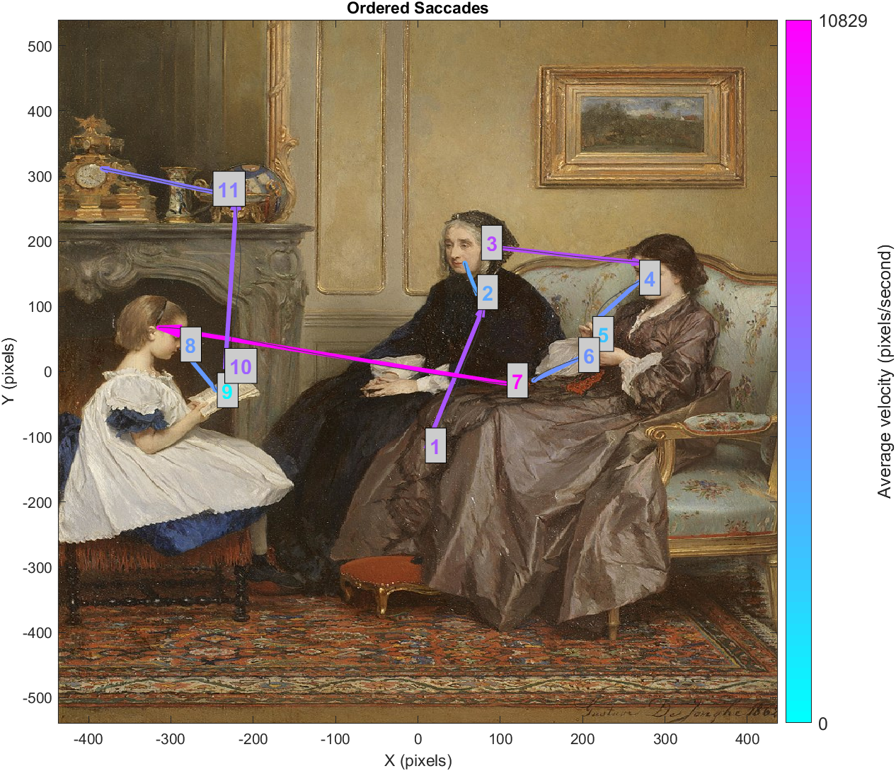
Plotting saccade data

Saccades are rapid movements of the eye between fixations. Like fixations, saccades are flagged automatically by the TRACKPixx3 recording. By default, saccade flags rise for eye movements faster than 10,000 pixels per second which last at least 10 frames. These criteria can be changed in PyPixx or MATLAB.

The final visualization in this project plots saccades as arrows that stretch from the average gaze location at  start of the saccade, to the average location at the end. The average raw gaze path is plotted in grey. Text labels correspond to the temporal order of saccades, while arrow and label colours indicate velocity.

As with our fixation data, we will save summary saccade data as a new field in our TrialData structure. We will also save the raw gaze paths while the saccade flag is high in a second field.

The first step to organizing saccades is very similar to how we organized fixations. That is, we will go into TrackerData and get the maximum of the left and right saccade flag columns. Then we will make lists of the beginnings and ends of our saccade events.

%let's combine right and left eye flags. We'll take the max of the two, meaning we assume a flag in 
%just one eye counts as a saccade. 
sacAvg=max([TrialData.TrackerData.LeftEyeSaccadeFlag, TrialData.TrackerData.RightEyeSaccadeFlag],[], 2);
%get our fixation starts and stops
saccadeStart = find((diff(sacAvg)==1)); 
saccadeStop = find((diff(sacAvg)==-1));
%if our participant started with a saccade, let's catch that and add a start on frame 1
if saccadeStart(1) > saccadeStop(1)
    saccadeStart=[1; saccadeStart];
end 
%if our participant ended on a saccade, let's catch that and add an end on max number of frames
if saccadeStop(end) < saccadeStart(end)
    saccadeStop=[saccadeStop; size(sacAvg,1)];
end 

Next, we’ll create a table to store our saccade data. We will also create a structure to store our average gaze paths during a saccade event.

We will loop through our list of saccade events and calculate the average of gaze locations for the two eyes, and the duration of the saccade. After calculating the 2-dimensional velocity between each frame in the saccade, we will get a single average velocity for the entire movement. We save this and our gaze path data.

%create a table with our saccade summary data, and a structure for our average gaze path
TrialData.Saccades = table();
TrialData.RawSaccadePaths = struct('x', [], 'y', []);
for k=1:numel(saccadeStart)
    %avg left and right gaze data
    x = mean([TrialData.TrackerData.LeftEyeX(saccadeStart(k):saccadeStop(k)),...
              TrialData.TrackerData.RightEyeX(saccadeStart(k):saccadeStop(k))],2, 'omitnan');
    y = mean([TrialData.TrackerData.LeftEyeY(saccadeStart(k):saccadeStop(k)),...
              TrialData.TrackerData.RightEyeY(saccadeStart(k):saccadeStop(k))],2, 'omitnan');
    duration = (saccadeStop(k)-saccadeStart(k)) * 1/2000;
    times = [TrialData.TrackerData.TimeTag(saccadeStart(k):saccadeStop(k))];
    %get mean velocity for the saccade
    vx = diff(x)./diff(times);
    vy = diff(y)./diff(times);
    vxy = sqrt(vx.^2 + vy.^2);
    avgVelocity = mean(vxy);  
    %add our data to a table and save the average trace for plotting
    TrialData.Saccades(k,1:3) = {k, avgVelocity, duration};
    TrialData.RawSaccadePaths(k).x = x;
    TrialData.RawSaccadePaths(k).y = y;    
end
%label our table so we can access it for plotting
TrialData.Saccades.Properties.VariableNames = {'Number', 'AvgVelocity', 'Duration'};

Now, time to plot, and save our results:

%plot
figure();
%plot our image as a background
image([plotRect(1), plotRect(3)],[plotRect(2), plotRect(4)], im);
hold on
%flip our y axis to correct for the inversion caused by the image function
ax = gca;
ax.YDir='normal';
%set axis limits to the boundaries of our image
xlim([plotRect(1), plotRect(3)]);
ylim([plotRect(4), plotRect(2)]);
xlabel('X (pixels)');
ylabel('Y (pixels)');
titlestr ='Ordered saccades';
title(titlestr);
%set some color map information
maxVelocity = ceil(max(TrialData.Saccades.AvgVelocity(:))); 
cmap = colormap(cool);   
for m=1:height(TrialData.Saccades)
    %get our arrow color. We'll scale everything to the maximum saccade observed and select a row
    %in our 64-row colormap based on this scaling.
    scaledVelocity = round((TrialData.Saccades.AvgVelocity(m)/maxVelocity)*64);
    scaledColor = cmap(scaledVelocity, :);
    %now we draw an arrow to represent the saccade path
    p1=[TrialData.RawSaccadePaths(m).x(1), TrialData.RawSaccadePaths(m).y(1)];
    p2=[TrialData.RawSaccadePaths(m).x(end), TrialData.RawSaccadePaths(m).y(end)];
    dp = p2-p1;
    quiver(p1(1), p1(2), dp(1), dp(2) ,0, 'LineWidth', 3, 'Color', scaledColor)
    %plot the gaze path itself
    plot(TrialData.RawSaccadePaths(m).x, TrialData.RawSaccadePaths(m).y, 'Color', [0.25, 0.25, 0.25]);
    %text label
    txt = int2str(m);
    text(TrialData.RawSaccadePaths(m).x(1)+5, TrialData.RawSaccadePaths(m).y(1)+5,txt,'Fontsize', 14,...
        'Color', scaledColor, 'FontWeight', 'bold', 'EdgeColor', 'k','BackgroundColor', [0.8,0.8,0.8])
end
%colour bar
c = colorbar('Ticks',[0,1],...
         'TickLabels',{'0',int2str(maxVelocity)},...
         'FontSize', 12);
c.Label.String = 'Average velocity (pixels/second)';
%some labelling and saving
save(datafile, 'TrialData');

Summary

In this project we covered four different methods of visualizing data from the TRACKPixx3. The TRACKPixx3’s accessible data output and automatic event flagging make it relatively easy to visualize the gaze data from a sample trial. 

We provided a sample dataset and gave some tips on formatting data for analysis. Next, we showed how to plot our visual stimulus as a background on our plot, and add raw gaze data as an overlay. We demonstrated generating a simple heat map, and creating labelled plots with fixation and saccade information. 

We hope these tools will serve as a jumping-off point for further data visualization and analysis. For even more visualization examples, including velocity plots and 3-dimensional plots of gaze path over time, please check out our TRACKPixx3 Demos.

Notes

The painting used in this project is “The recital” by Gustave Léonhard de Jonghe. This image is considered public domain and can be freely reproduced. Image file courtesy of Wikimedia Commons.