
Many vision science experiments are also auditory experiments. You may play a tone to prompt a response, play audio and visual stimuli concurrently to measure their contributions to perception, or otherwise compare visual and auditory processing performance.
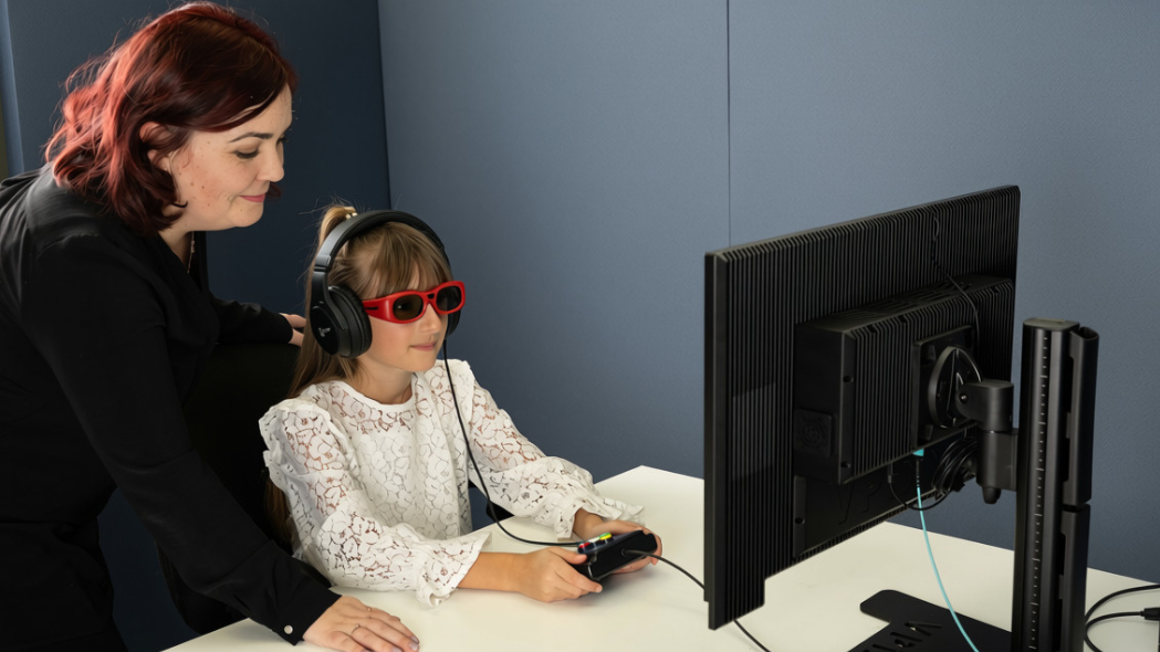
Whether you are in a magnetically shielded environment or a behavioural laboratory, audio stimulus timing deserves careful consideration when designing your experiment.
VPixx devices offer a unique audio delivery mechanism that synchronizes audio with display behaviour at microsecond precision. For studies where audio timing is critical, this offers a solid advantage over audio timing controlled by standard methods like a PC soundcard.
In this guide, we will discuss how to present auditory stimuli using the audio subsystem built into VPixx data acquisition hardware. By the end of the guide you will understand how to configure, upload, and drive audio output from our system, optionally synchronized to video output.
We include examples in MATLAB and Python, and conclude with a short discussion of auditory level equalization.
We assume you are familiar with the basic logic of VPixx hardware control, including device registers, the local register cache, and schedules. If not, we recommend starting with this guide: The Logic of VPixx Hardware Control.
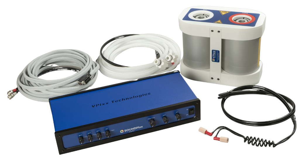
Two ways to control audio in your experiment
If you have a VPixx system, there are two methods to convey audio to your participant:
-
From the computer's sound card, using the audio facilities of your experiment software (e.g., PsychPortAudio in Psychtoolbox, or the sound libraries in PsychoPy)
-
From your VPixx hardware, by uploading waveforms to device memory and playing them through the onboard audio codec with a hardware schedule.
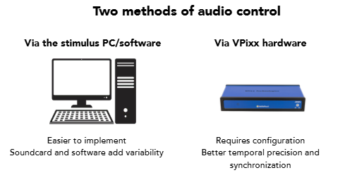
If your study needs consistent audio onset timing, and especially if it needs sound aligned to what is on the screen, we recommend you play your audio from the VPixx hardware. If audio timing precision isn’t critical (e.g., playing movies), the soundcard is usually sufficient and easier to set up.
To play audio from the soundcard, simply connect the speaker jack directly to your PC and use your standard playback controls in software.
The remainder of this guide focuses on how to implement precise audio control and audio/visual synchronization using VPixx hardware.
Playing audio from VPixx hardware
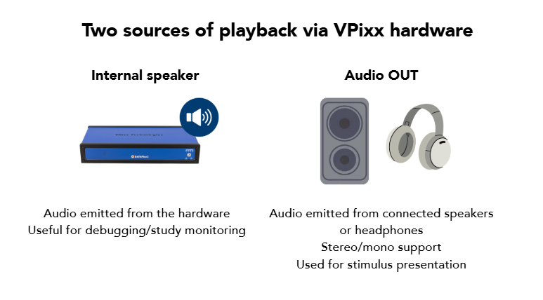
We will demonstrate how to drive audio from our system using a concrete example of playing a tone. First, you will need to connect powered speakers or headphones to the Audio OUT 3.5 mm stereo jack of your VPixx device (see below).
VPixx devices with audio support include:
-
DATAPixx series I/O hubs
-
VIEWPixx 12-bit and VIEWPixx /3D systems
-
PROPixx controller
Depending on the age of your device, you may have a ‘full’ or a ‘lite’ system. Only full systems have audio support. Units sold after September 2023 are all ‘full’ systems. See https://docs.vpixx.com/faq/hardware#What-is-the-difference-between-a-%E2%80%9CLite%E2%80%9D-and-a-%E2%80%9CFull%E2%80%9D-data-acquisition-system? for more details.
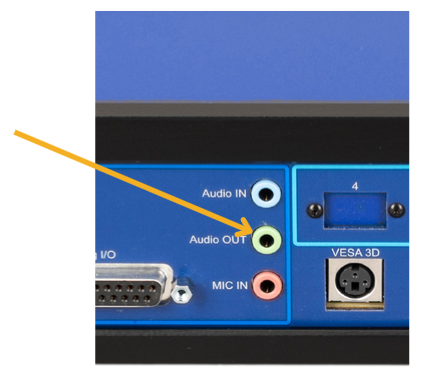
You will also need to ensure the VPixx device is connected to the stimulus PC via USB. If you are using a DATAPixx I/O hub and plan to synchronize with video, you will need to ensure the video signal is routed through the hub. See https://docs.vpixx.com/hardware/datapixx3#Product-assembly---Connecting-the-stimulus-and-console-display for more details. Note that on our VIEWPixx LCD screens and PROPixx controller, video integration is built-in.
The process to generate and play a tone has five steps, with the same workflow in both MATLAB and Python:
-
Generate your audio waveform in the host software, as floating-point values between −1 and 1.
-
Initialize the audio codec for the hardware (once per session) and set the volume.
-
Write the prepared audio waveform to the VPixx device memory using an audio buffer write.
-
Configure a playback schedule: set parameters like onset delay, sample rate (8000–96000 Hz), number of frames, and left/right channel.
-
Start the schedule. Nothing happens on the device until a register write pushes your staged commands. This is what makes the synchronization described in the next section possible.
Click on the sections below to expand code examples for our Python and MATLAB APIs.
Why load waveforms onto hardware? Putting sound files on our dedicated hardware means we can control playback with fully deterministic timing. While the setup requires a bit more work, the tradeoff is tightly-managed audio and trustworthy stimulus timing.
For stereo playback, you can pass a two-row waveform (row 1 = left, row 2 = right) to the buffer write, and use lrMode 3 (MATLAB) or 'stereo1' (Python). Mono mode sends the same samples to both ears.
For sounds too long to fit comfortably in memory, we suggest you write an initial block, then top up the buffer during playback (MATLAB address argument −1 appends at the current write pointer) while polling the audio status field freeBufferFrames. For more advanced techniques for continuous streaming, see the demo https://docs.vpixx.com/matlab/streaming-continuous-audio.
Adjusting the volume
You can adjust your waveform volume by scaling the waveform digitally (e.g., scaling an output of 0.5 → 0.25 to make it quieter) or adjusting the speaker volume knob. You can also set a master volume level in our codec.
When designing your experiment, the audio system must preserve both signal resolution and setting replication. We recommend configuring your waveforms and any knobs or dials to a fixed level across the study, and using the codec settings to finely and systematically control volume for within-study volume manipulations.
To preserve audio levels with good resolution and replicability:

1. Set waveform intensity ->
2. Lock in any physical dials ->
3. Use the codec volume for fine-tuning
You can digitally scale your waveform using (Datapixx('SetAudioVolume', v) / DPxSetAudVolume(v)). This is a helper function that scales your waveform samples digitally on a linear 0–1 scale.
To set the codec volume use DPxSetAudCodecOutVolume in Python and SetAudioVolume with source=1 in MATLAB. This attenuates audio in the codec hardware. Attenuation can be expressed linearly or in dB (0 to −58.5 dB; −59 dB and below is mute).
The audio codec volume control also distinguishes the Audio OUT jack from the hardware’s internal speaker, and left from right sound sources. You can set each independently (e.g., mute the built-in speaker while driving headphones).
Aligning audio and visual onsets
Playing a sound and flipping the screen in adjacent lines of code does not make them simultaneous. To fully align what the participant hears with what they see, you need to characterize the presentation timing and account for channel-specific delays.
Audio timing from "the schedule started" -> "sound arrived at the ear"
Video timing from "the flip command" -> "light left the display"
The following sections walk you through the known signal timing delays in both channels, and shows how to configure audio playback to precisely map to physical display output.
Characterizing the audio timing
-
Codec group delay. The audio codec's digital filters impose a short, sample-rate-dependent delay between when a schedule sends a sample and when that sample peaks at the Audio OUT jack. Our helper functions allow you to determine it for your target sampling rate:
For example, the group delay of the codec for a common sampling rate of 44100 is 0.50 ms.
-
Transducer group delay. Electrical speakers and pneumatic transducers impose a second group delay when they convert the audio signal into sound waves. You can measure this with an area microphone placed directly at the transducer or speaker opening, and a series of tone sweeps. Group delay is computed as
 from the unwrapped phase after 1/6-octave smoothing. We have measured this delay for the SOUNDPixx pneumatic transducer and report it below. Group delay is not constant across frequency; it is several milliseconds near the low-frequency resonance and falls to about 0.3 ms above 1 kHz. As such, we report delay across two example bands. Across the working band (100 Hz–2 kHz) it is 0.89 ms, and within a typical 500 Hz–2 kHz tone-paradigm band 0.78 ms. The absolute value includes the few centimeters of mic air-gap and is best read as an upper bound on the transducer's intrinsic delay.

-
Sound transmission delay: Once sound leaves the transducer or speaker, it travels through air to reach the ear. Longer distances between the sound source and the ear can impose a transmission delay. MRI-safe headsets such as the SOUNDPixx place the transducer outside the bore and pipe the sound to the ears through air-filled tubes, which adds measurable latency to the signal arriving at the ear. The whole air path includes the 3.7 m main tubing plus the ~1.4 m headphone tubes. Sound in air travels at roughly 343.50 m/s at 20 °C, so the tube adds:

14.73 ms is nearly two full frames at 120 Hz, and represents the most substantive delay in the audio pipeline.
Characterizing video timing
Register writes can lock commands to synchronize with video events:
-
Datapixx('RegWrVideoSync')executes your staged commands on the next vertical sync, and -
Datapixx('RegWrPixelSync', pixelTrigger, timeout)executes them when a specific pixel sequence is detected in the video signal (Python:DPxWriteRegCacheAfterVideoSync(),DPxWriteRegCacheAfterPixelSync()).
Pixel Sync is the more robust of the two, because it fires on your actual stimulus content rather than on a frame boundary that is vulnerable to frame dropping. For more details on Pixel Sync and the frame delays for each of our displays, see our guide to Pixel Sync.
Example: psync-locked audio through a pneumatic headset
In this example we drive the PROPixx at 120 Hz and play a 500 Hz tone using the SOUNDPixx pneumatic in-ear earphones with standard 5.055 m total air path, and sampling rate of 48 kHz.
We want sound to arrive at the ear at the moment the stimulus illuminates.
-
When does the stimulus illuminate?
If the psync trigger pixels are embedded in the stimulus frame, the PROPixx illuminates that frame one frame period after its data begins. At 120 Hz a frame period is 8.33 ms. -
How long does the audio path take? Group delay computed by our function + estimated transducer delay from specifications + tube length divided by speed of sound = 0.46 + 0.78 + 14.73 = 15.97 ms after the schedule starts.
-
Compare. Because the audio delay is longer than the video delay, the audio must start first.
-
Launch one frame earlier. Put the psync pixels one frame before the stimulus appears so the video delay is 16.67 ms. Then compute an audio schedule onset based on the new psync time:

The general rule: if audio lead time exceeds the display's illumination delay, start the schedule on an earlier frame and add whole frame periods until the schedule onset can be a positive value.
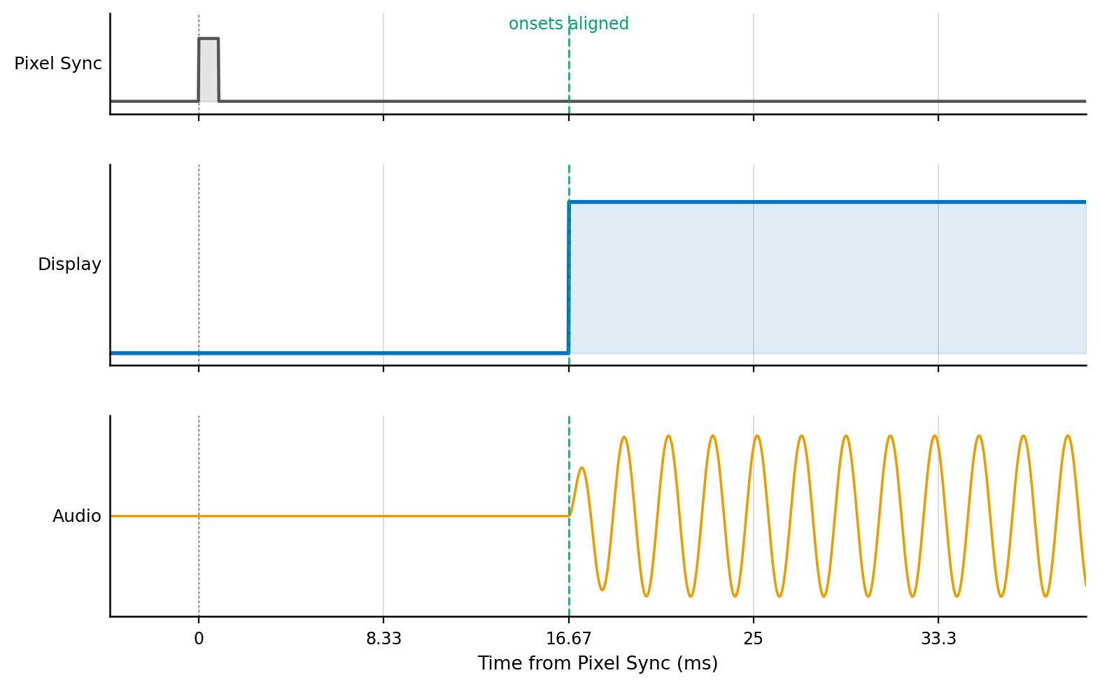
Consider ramping audio onset. A tone that jumps from silence to full amplitude in a single sample contains a step discontinuity: a broadband "click" (spectral splatter) that is audible, contaminates your intended spectrum, and can drive the codec or amplifier into distortion. Apply a short amplitude ramp (a few ms cosine/Hann window) at the start and end of every sound. This slightly softens the very first instant of the onset, so if you need sub-millisecond onset precision, define your "onset" as a fixed point on the ramp (e.g., its midpoint), adjust your scheduleOnset to match, and keep the ramp duration constant across trials.
Keeping volume consistent across frequencies with equalization
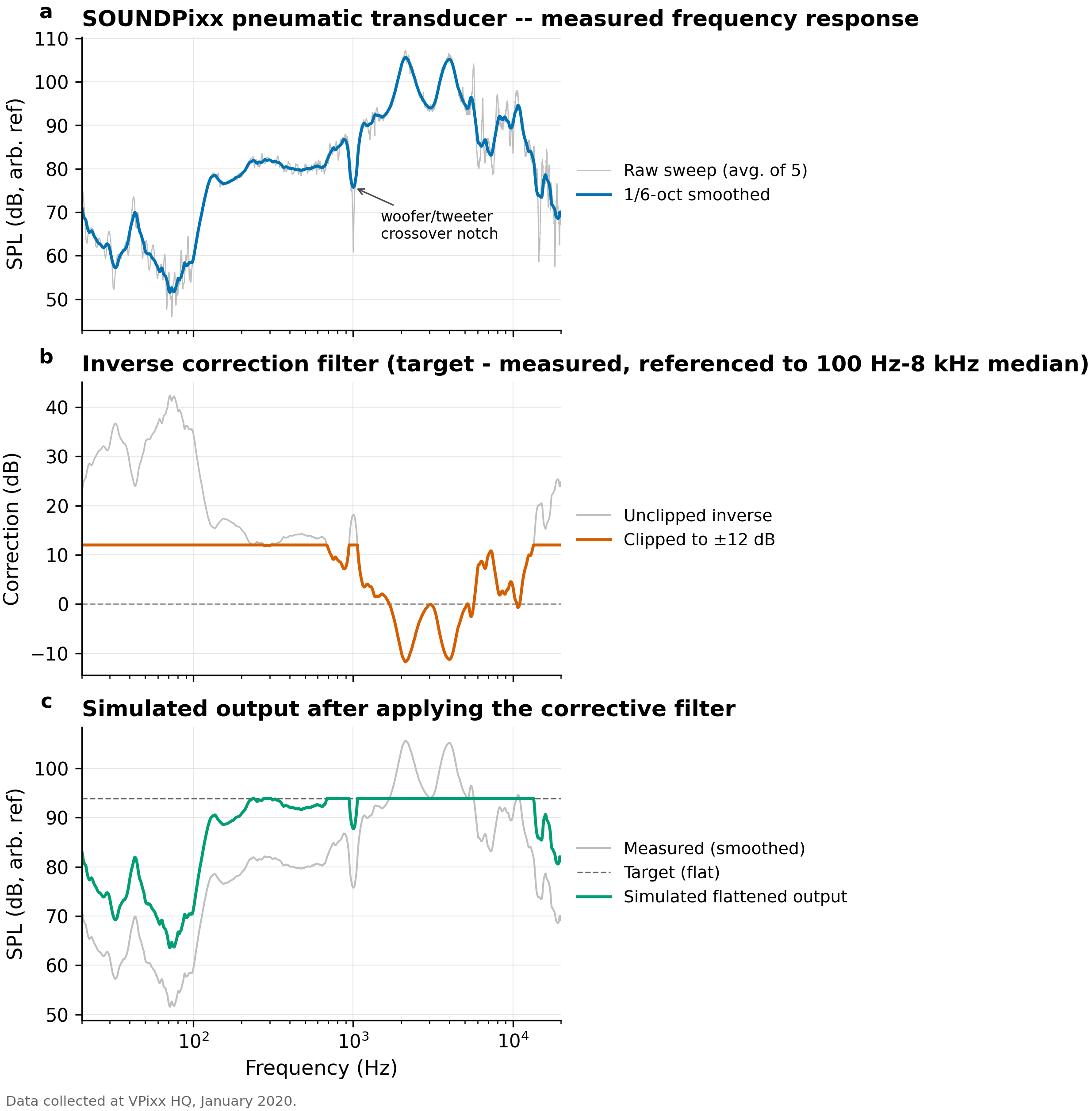
No transducer has a perfectly flat frequency response. The speakers and headphones act as acoustic filters, with resonances and roll-offs that can shift the level of one tone relative to another by many dB. Consider the frequency response of the SOUNDPixx (see a below). The attenuation in high frequencies is typical of a pneumatic system:
There is an entire hobby dedicated to identifying audio systems with the ‘best’ frequency response profile for different types of music. A fully flat frequency response is ideal for research, as it ensures that setting and changing stimulus volume is consistently applied regardless of the target frequency.
Consider an oddball paradigm with a high tone and a low tone. Simply setting the volume of each tone to 50% doesn’t mean they will have the same audio output. Your participants may react to one stimulus more strongly simply because it is physically louder given your specific audio system’s frequency response profile.
Equalization is the process of dynamically adjusting output volume to account for a sound system’s given frequency response profile. Equalizing a system to a flat output requires:
-
Measuring what actually arrives at the ear, using a calibrated microphone at the ear end of the system, driven with known test signals
-
Generating an inverse correction that boosts what the system attenuates and cuts what it resonates, typically applied at the software level.
The freeware standard for the measurement-and-inverse workflow is Room EQ Wizard (REW). You must measure the transfer function with an audio sweep, inspect the magnitude response, and export correction filters. A detailed walkthrough is beyond this guide's scope; the practical takeaway is that equalization is a per-system calibration. It must be re-checked when tubing or ear tips change. For quantitative auditory work, it is highly recommended as a calibration step for your audio system.
Equalization has hard limits. An inverse filter cannot create energy the system cannot transmit. Thus, "boosting" an attenuated band really means cutting everything else down to meet it. Depending on your audio system, flattening the response to match the weakest high-frequency band leaves the whole stimulus set very quiet. For some systems, like pneumatics, the sensible compromise is to equalize only across the frequency range your paradigm actually uses and accept a roll-off above it (see b and c above).
Equalization does not account for the unique filtering properties of individual human ears. Thus, while equalization can flatten the sound output that reaches the ear, it does not guarantee each individual will perceive the same volume across all frequencies. In-ear headphones are best to avoid the largest individual filters (the pinnae or outer cartilage of the ear) but even then, individual differences exist.
The next generation of SOUNDPixx3 will have a built-in equalization function for flat audio output. Current SOUNDPixx users can get in touch with us for tips on how to equalize their existing systems.
Summary
In this guide, we covered how to use your VPixx hardware to control audio output precisely in your experiments. We discussed how and why to upload audio waveforms to your hardware, control volume, trigger playback, and optionally compute and correct for audio and visual channel delays to achieve true audio-visual synchronization. We ended with a short discussion of audio equalization and why it matters for every sound system used in audio research.
We hope this guide has empowered you to evaluate and implement your own auditory stimulus presentation pipeline. Have questions about our hardware, or want to know more? Drop us a line at support@vpixx.com.
Related resources
-
Playing audio and Streaming continuous audio — MATLAB demos
-
AudioOut class reference and libdpx wrapper — Python demos
-
SOUNDPixx — user manual
-
Room EQ Wizard — third-party measurement and correction software