Synchronization Strategies for Multimodal Neuroscience

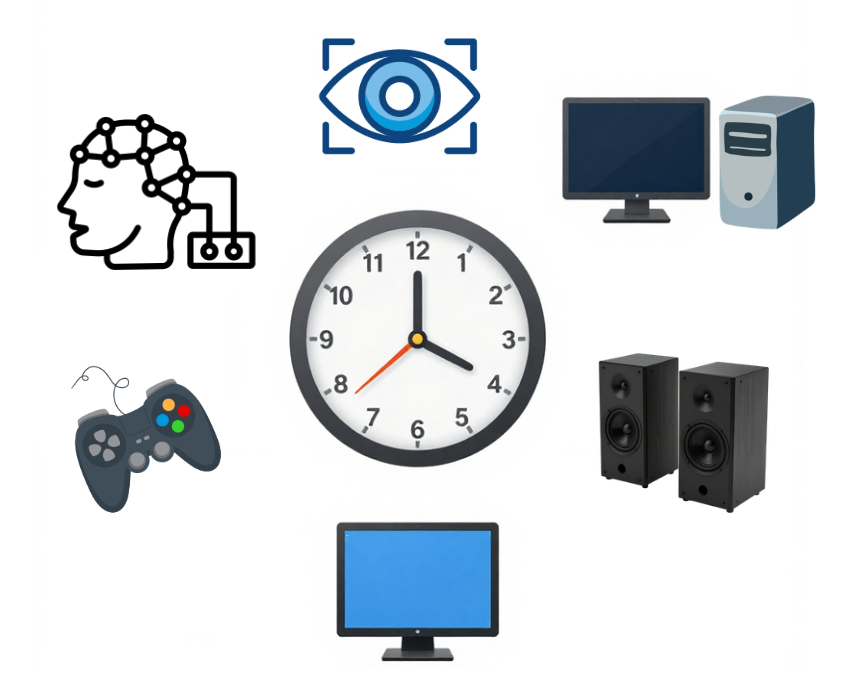
Modern neuroscience experiments routinely combine multiple data streams: visual stimulation, neural recording (EEG, MEG, OPM-MEG), eye tracking, physiological measures, response collection, and more. Each recording device has its own clock, its own sampling rate, and its own pathway from physical event to recorded data point.

It is a major design consideration how to align all of these streams, or synchronize them, onto a common timeline with sufficient precision for your scientific question. There is no single "best" synchronization approach; the right method depends on the timing tolerance your specific analysis requires. Do you need precision in the milliseconds, or microseconds?

For instance, a cognitive pupillometry study averaging across 500 ms epochs has very different synchronization needs than a microsaccade-locked ERP analysis or a gaze-contingent display paradigm. There are also practical considerations, such as the need to purchase dedicated cabling or hardware, vs. open-source software-based solutions.

This guide discusses five common data timestamping and synchronization strategies in multimodal neuroscience. For each strategy, we explain the method and principles behind it, discuss the consequences for timing precision, and consider the strengths and weaknesses in practice. This is followed by a general discussion of timing uncertainy budgets and clock drift, which is a concern for longer studies.

By the end of this guide, you should feel empowered to make experiment hardware and software design choices aligned with your specific research needs. This document is not a ranking. Different synchronization strategies serve different end goals. The best design depends on your lab’s resources and the kind of research you do. We provide this information simply to help scientists understand the engineering behind data acquisition timing and synchronization, so they can make the best choice for their research.

Within-Stream vs. Cross-Stream Timing

First, we need to distinguish between two different kinds of temporal precision.

Within-stream precision is the timing quality of a single data stream in isolation — how evenly spaced are the samples, how accurately does each timestamp reflect the moment of acquisition, and how stable is the sampling clock over time. A well-designed device with a dedicated clock (whether a real-time operating system, a crystal oscillator, or a field-programmable gate array) can achieve excellent within-stream precision. An EEG amplifier sampling at 1024 Hz with a stable crystal clock produces evenly spaced samples with low jitter. An eye tracker running on a dedicated host PC timestamps its gaze samples with high internal consistency. Within-stream precision is what manufacturers typically report on their spec sheets.

Cross-stream precision is the timing quality of the alignment between two or more data streams — how accurately can you say that gaze sample A and EEG sample B correspond to the same moment in time? This is a more difficult problem because it depends not on any single device's clock quality but on the relationship between clocks that are, in general, independent. Cross-stream precision is limited by the synchronization method used to bridge the devices. These are the methods we will discuss below.

Something to keep in mind while reading this guide is that these two kinds of precision are separate but compounding. A system can have excellent within-stream precision and poor cross-stream precision. For example, two devices with high-speed internal clocks can drift relative to each other because they have no shared timing reference.

Conversely, a system with mediocre within-stream precision (e.g., USB-polled at variable intervals) cannot be rescued by even the best cross-stream synchronization, because the individual timestamps are imprecise to begin with.

The total timing uncertainty in any multimodal experiment is the combination of both the within-stream jitter of each device, plus the cross-stream synchronization error between them. The five strategies described below primarily address the cross-stream problem (how to bridge independent clocks) but their effectiveness is always bounded by the within-stream quality of the devices being bridged.

Five Common Synchronization Strategies

1. TTL Digital Triggers

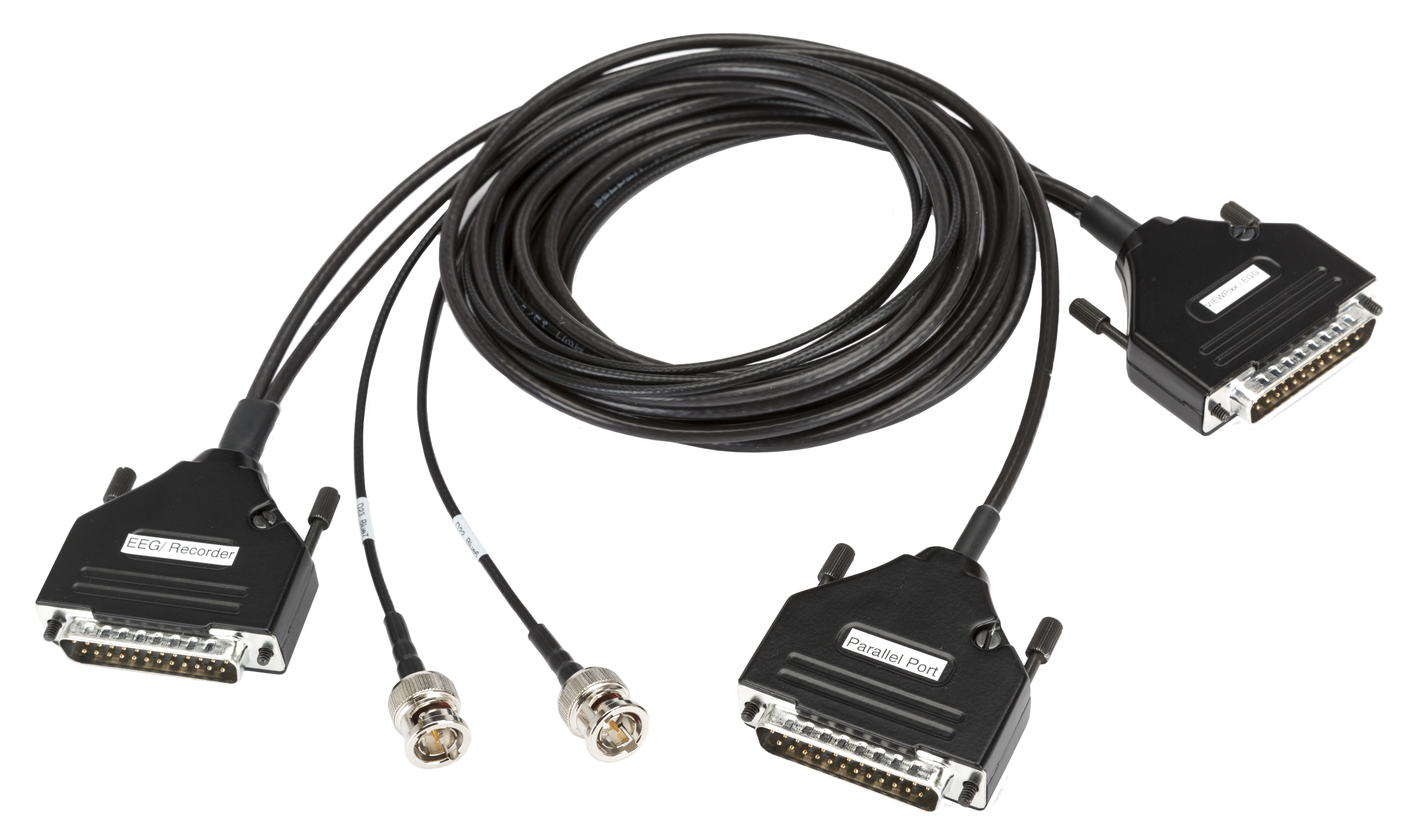
The oldest and simplest method to align data streams is a synchronization pulse on a wire. A TTL trigger is a simple binary voltage transition that marks the occurrence of an event. Electrical propagation is essentially instantaneous (nanoseconds), making the signal as close to zero-latency as physically possible. This type of trigger is the primary method of MR signalling, but it is also used by other systems. This is the method we use for Pixel Mode video triggers.

How it works

The sender asserts a voltage change via a physical connector, typically a parallel port or BNC port, at a specified moment (e.g., stimulus onset). This signal is wired directly into the receiver’s trigger input, where it is sampled at the receiver’s native rate and timestamped by its local clock. The result is a shared marker that reliably marks an event on the sender side (e.g., stimulus presentation) directly in the receiver’s data stream (e.g., eye tracking recording).

Timing characteristics

The electrical propagation delay of a TTL pulse through a short cable is negligible (nanoseconds). Timing uncertainty comes not from the trigger itself, but from the end points: the sender's temporal precision, and the receiver's acquisition fidelity.

If the trigger is sent from software (e.g., immediately after a PsychoPy or Psychtoolbox flip command), the OS thread scheduler can introduce jitter, typically on the order of tens to hundreds of microseconds, with occasional spikes of a millisecond or more. This jitter occurs before the electrical signal is even generated, adding to the net imprecision of the system synchronization.

Hardware matters too. Parallel ports are generally faster (~1 µs write latency) than USB-to-TTL adapters, which show 0.15–0.40 ms jitter (ANT Neuro, 2025).

One way to avoid this jitter is to use dedicated triggering hardware and lock TTL pulses to known events that are detected at high speeds. Systems like the DATAPixx3 can schedule TTL triggers in advance, or lock their onset to video events with deterministic timing. This strategy bypasses OS-level jitter altogether.

Generally speaking, TTL communication should flow from the system with the best signal generation timing to other systems. Sometimes, in practice, this is not possible; for example, MR triggers typically send sync pulses and cannot receive them.

It is important to remember that signal precision does not equate to physical alignment with events, even for hardware-locked triggers; for instance, due to the video transmission pipeline, PROPixx Pixel Mode triggers lead physical screen illumination by precisely 1 frame. Consistent offsets are not an issue if they are corrected for in post-processing. It is the variability that matters for final data fidelity.

Strengths and limitations

TTL triggers are simple, well-understood, and nearly universal. Virtually every EEG amplifier, MEG system, and eye tracker has a TTL input. The final synchronization precision is primarily determined by the precision of signal generation (by the sender) and the acquisition fidelity (by the receiver).

TTL’s simplicity is also its limitation. TTL signals carry limited information and can only mark discrete on/off events, not continuous data streams. They also require a physical connection between systems.

2. Polling via USB

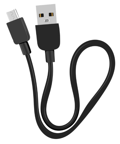
Many modern neuroscience peripherals, including eye trackers, EEG amplifiers, response devices, and physiological sensors, connect to the host computer via USB. Some researchers treat USB as a synchronization pathway, using the host computer's clock to timestamp incoming data and outgoing events alongside managing experiment timing. This is how mouse and keyboard events are polled.

How it works

A USB device sends data to the host in periodic packets determined by the device’s polling interval. For most research devices, this is 1 ms (1000 Hz), meaning data is transferred in discrete bursts at 1 ms intervals. The host’s USB controller schedules these transfers, and the operating system processes them through interrupt service routines (ISRs) and deferred procedure calls (DPCs).

Timing characteristics

The USB polling interval creates a fundamental quantization of timing: any event that occurs between polls cannot be timestamped more precisely than the polling interval. With a 1 ms poll, this means up to 1 ms of latency on every transfer, with the actual delay depending on where in the polling cycle the event occurs. On top of this, OS scheduling jitter adds variability. Under normal conditions, this is small (tens to hundreds of microseconds), but under CPU load, it can spike significantly. Psychtoolbox documentation notes that some USB DAQ devices exhibit occasional latency spikes of 10–20 ms.

USB 3.0+ devices can achieve sub-millisecond polling intervals (down to 125 µs microframes), but this depends on the specific device firmware, host controller, and OS driver stack, and is therefore vulnerable to the above mentioned latency spikes.

Strengths and limitations

USB is convenient and ubiquitous. Whereas TTL only marks discrete events, USB can stream rich contextual data. The tradeoff is that it inserts the operating system into the timing path, making every timestamp dependent on OS behaviour. The consequence is that USB timing is only as good as the host computer's ability to service interrupts promptly, which varies with CPU load, driver quality, power management settings, and other factors that are difficult to control across labs.

This does not mean that USB polling has no place in high-precision systems. For instance, our DATAPixx3 communicates with the experiment PC via USB, and this is the primary method for fetching moment-to-moment data, e.g., to update a gaze contingent display or log a button press to continue to the next trial. In cases like these, the timestamping is done on dedicated hardware, and the latency/variability is tied to real-time import via USB— typically fine for dynamic experiment management, but postprocessing uses the hardware timestamps to preserve hardware-based precision.

3. Ethernet (Direct or Networked)

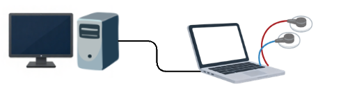
Some devices use a dedicated Ethernet link between a dedicated device PC using a Real-Time Operating System (RTOS) and a separate stimulus/experiment PC driving the experiment. This architecture decouples the timing of device logging from that of the general-purpose stimulus computer, yielding robust, high-speed event timestamps. Syncrhonization is managed by Ethernet communications between the two systems, which is a fairly high-speed and information-dense communication protocol.

How it works

In this architecture, the acquisition device (e.g., an eye tracker or high-channel-count amplifier) connects to a dedicated “device PC,” running a stripped-down, real-time or near-real-time operating system. Data is computed and timestamped entirely on this dedicated device. The Ethernet link between the device PC and the experiment PC can be used to poll data from the device PC (e.g., for online experiment updates) and send messages to the device’s data stream.

Event messages from the stimulus PC are timestamped by the device PC's clock upon arrival, and typically, the transmission delay is recorded for post-hoc correction.

To synchronize data with external recording devices (EEG, MEG, etc.), these systems may also support TTL triggers via the parallel port on the device PC (see strategy #1 above).

Timing characteristics

Dedicated Ethernet architectures typically achieve real-time data availability to the stimulus PC with end-to-end delays in the low single-digit millisecond range. The data timestamps themselves are highly precise because they are assigned by the device PC's real-time OS at the moment of acquisition, with minimal scheduling ambiguity.

The timing consideration arises in event message timestamping. The event messages that link the two PCs are generated by the stimulus computer's OS, which means the triggers inherit the stimulus computer's scheduling jitter— typically sub-millisecond, but variable, as discussed in strategy #2.

There is also a concern about drift. Between messages/TTL triggers, the device PC's clock and the experiment PC clock run independently and may drift relative to each other (see the Clock Drift section).

Strengths and limitations

A dedicated device PC running a real-time OS is a strong solution for acquiring high-speed data — timestamps are clean and deterministic. Messages passed between the device and stimulus PC are rapid, but message generation driven by software inherits OS jitter. TTL-based co-registration with external devices can close this gap with precise event-locked triggers. Clock drift between parallel PCs is something to keep in mind, particularly for longer acquisition periods. The practical implementation of having a dual-PC setup must also be considered; researchers need to switch between two distinct PCs and operating systems, and manage both in parallel, which adds to operational overhead.

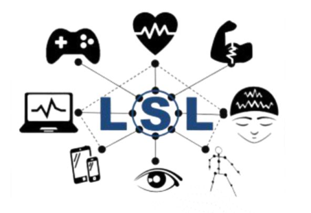
4. Network Software Synchronization (Lab Streaming Layer)

The Lab Streaming Layer (LSL) is an open-source middleware for unified collection of time-series data across any number of devices over a local area network. Its clock synchronization protocol, modeled after the Network Time Protocol (NTP), estimates and corrects clock offsets between machines (LSL documentation).

How it works

Each device runs a small program (an "outlet") that pushes timestamped samples to the network. A recording application (typically LabRecorder) discovers all outlets and records their data into a single XDF file. Clock offsets between machines are periodically measured via round-trip time exchanges, addressing clock drift over time. Post-hoc, the XDF importers for MATLAB and Python apply offset correction and optional jitter removal to align all streams to a common timeline.

Timing characteristics

LSL's own documentation states that local (same-machine) transport latency is typically under 0.1 ms. Cross-machine clock synchronization achieves an inter-device offset jitter (standard deviation) of approximately 145 µs under controlled conditions (Kothe et al., 2025). However, the total timing uncertainty for any given data stream includes the device's own latency and jitter (USB transfer, device buffering, driver processing), the OS timestamp quality, and the network transport delay. Importantly, the LSL authors state explicitly that LSL "does not have access to any incoming data until the moment it is received by the CPU" and therefore "cannot itself learn or estimate whatever on-device delays within each recording device occurred" (Kothe et al., 2025, Section 1.2). These device-specific setup offsets were measured at 6–12 ms for a BioSemi amplifier in their benchmarks, and the authors note that total device delays, including on-device buffers and wireless transmission, can add up to several tens of milliseconds. Brain Products has reported that total end-to-end latency can range from a few milliseconds to approximately 100 ms, depending on the specific device and setup configuration.

The LSL authors also demonstrated that their built-in jitter correction (dejitter) achieves sub-millisecond synchronization between professional-grade devices with uniform sampling rates; however, this correction breaks down for consumer-grade or irregularly-sampling devices such as webcams, where disabling jitter correction actually improved alignment (Kothe et al., 2025, Section 3.3).

Strengths and limitations

LSL's strength is flexibility and universality. It supports over 150 device classes, works across platforms and programming languages, handles connection recovery gracefully, and provides a unified file format for multi-stream data. For recording many heterogeneous streams with minimal setup effort, it is a fantastic solution.

Its limitation is that it operates on top of every other source of timing uncertainty in the chain. LSL does not replace or bypass USB polling jitter, OS scheduling variability, or device-internal buffering — it adds its own (small) uncertainty on top of these. As the LSL authors themselves recommend, researchers should measure setup offsets for all devices and configurations before recording experiment data. This reintroduces operator load in the form of system calibration, which must be repeated with each change to the system configuration or experiment software.

5. Dedicated Hardware Clock (FPGA-Based)

At the highest precision tier, dedicated hardware I/O hubs eliminate the OS, the network, and the USB bus entirely from the timing path. Rather than solving the synchronization problem after the fact, this approach avoids it by design: a single field-programmable gate array (FPGA) provides one clock domain that timestamps multiple recorded data streams simultaneously. The supported data types depend on the hub. For instance, the DATAPixx3 can record audio, analog, digital and eye-tracking data (from the TRACKPixx3) to its onboard memory. See the DATAPixx3 user manual for details. It can also configure its audio, analog, and digital outputs to lock to a simultaneously emitted TTL synchronization pulse for alignment with unsupported data streams.

I/O hubs are not waystations in experiment design, but rather a hardware backbone for experiment timing. They replace OS-based timestamping with a dedicated system designed for precision recording and signal generation. Video-monitoring hubs also ‘listen’ to video passed through the hardware and can lock TTL and I/O recording/playback to events detected in the video stream after it leaves the graphics card. If the properties of the display engineering are known, this becomes another microsecond-precise method of event detection.

It is worth noting that Psychtoolbox, the most widely used stimulus presentation software in vision and cognitive neuroscience, uses the DATAPixx hardware clock as ground truth when evaluating the precision of its own software-reported flip timestamps. This independent adoption of FPGA-based timing as a reference standard reflects the broader principle: hardware clocks serve as the benchmark against which software and OS-based timing is measured.

How it works

The DATAPixx3 contains an FPGA that provides a single high-precision 100MHz master clock. This clock simultaneously drives video timestamping, digital I/O (TTL triggers to/from amplifiers, including video-locked triggers), analog I/O (physiological signals, reference waveforms), audio I/O, and, when paired with TRACKPixx3, eye tracking. All of these signals share the same clock domain with sub-microsecond alignment. Data is buffered on-device and retrieved by the host computer in bulk, but the timestamps are assigned by the hardware at the moment of acquisition, not by the host OS.

Critically, the TTL triggers that the DATAPixx3 sends to external devices (EEG amplifiers, MEG systems) are generated by the same FPGA clock that timestamps the stimulus onset and the gaze data. This means that even the signals leaving the VPixx ecosystem are time-aligned with the master clock. The receiver still has its own clock, but the trigger it receives is hardware-precise and deterministic, regardless of what the host computer's OS is doing at that moment.

Timing characteristics

Because all signals share a single hardware clock, there is no synchronization problem to solve between them. The alignment between a stimulus onset event, the corresponding gaze sample, and the TTL trigger sent to your amplifier is deterministic and intrinsic — it does not need to be estimated, corrected, or calibrated. The timing precision is governed by the FPGA clock rate (sub-microsecond), not by OS scheduling, USB polling, or network transport.

Strengths and limitations

This approach provides the highest possible timing precision and the simplest synchronization model. It is also the most robust: timing precision is invariant to host CPU load, network conditions, operating system, or software configuration. The system integration aspect means that adding eye tracking (TRACKPixx3) to an existing DATAPixx3 setup does not introduce a new clock domain or a new synchronization problem — the gaze data is simply another signal on the same hardware.

The limitations are the cost (of a high-end dedicated hardware system vs. free options like LSL) and scope: the hardware clock directly covers devices connected to the FPGA. For devices that cannot be directly connected (e.g., a motion capture system in another room), you still need an external synchronization method (TTL triggers or LSL) to bridge to the external device. VPixx offers a catalogue of TTL cables for third-party systems to facilitate this integration, and we also provide custom cabling. Because the DATAPixx3's TTL triggers are themselves hardware-clocked, the TTL synchronization bridge inherits the FPGA's timing precision.

Comparison at a Glance

Note: The jitter values above are representative ranges based on published measurements. Actual performance depends heavily on specific hardware, drivers, OS configuration, and network conditions. The values for LSL reflect cumulative end-to-end uncertainty, including device-side contributions, not just LSL's own transport layer.

The Timing Uncertainty Budget

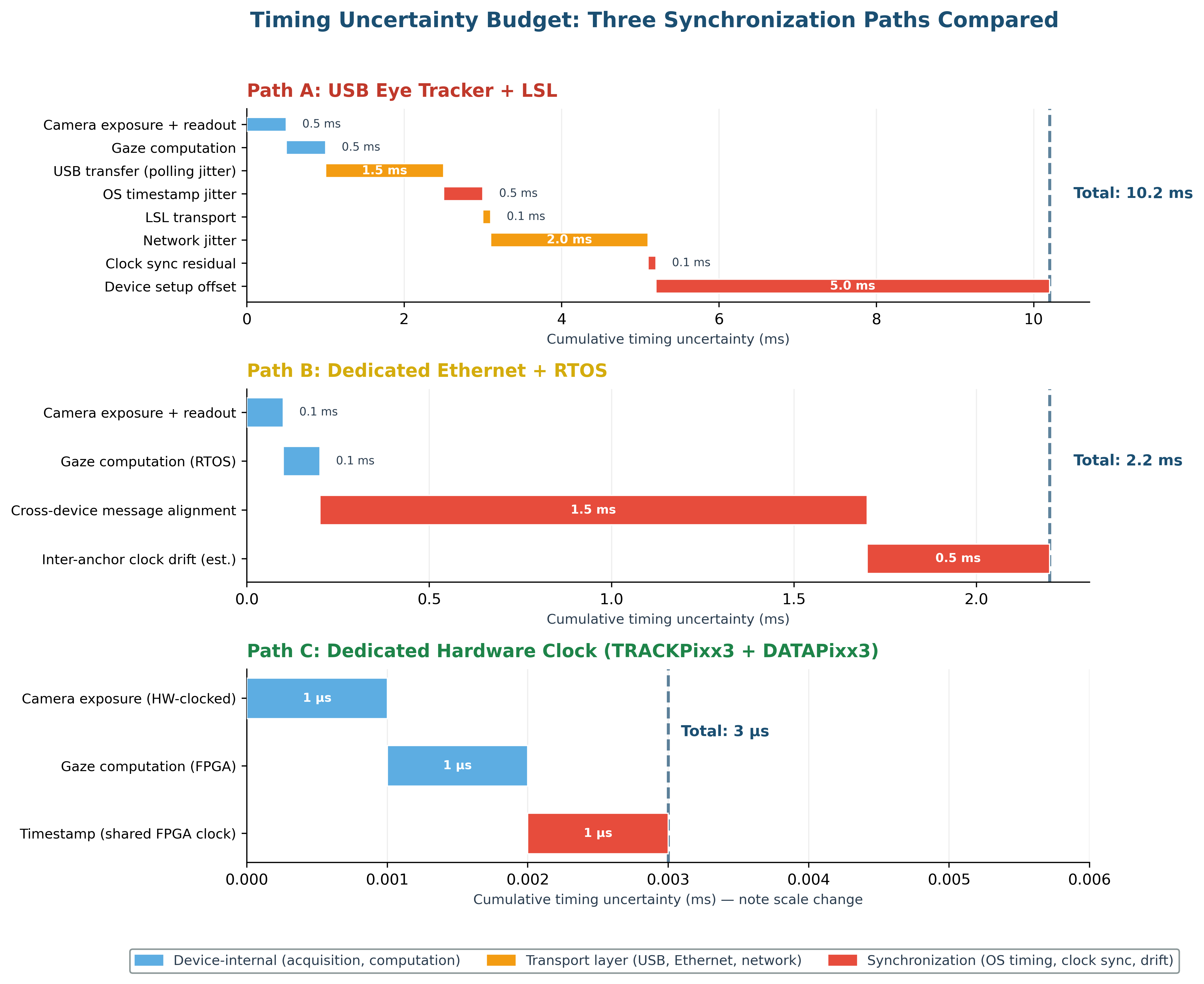
A useful way to evaluate any synchronization approach is to trace the timing uncertainty budget — the sum of all timing errors that accumulate between a physical event and the timestamp that represents it in your data file. Here we walk through this budget for a concrete example of a two-stream synchronization: aligning eye tracking data with stimulus events.

A note on latency vs. jitter: It is important to distinguish between latency (a constant, fixed delay in the signal path) and jitter (the variability of that delay from sample to sample). A constant latency — even a significant one — does not degrade synchronization, because it shifts an entire data stream by a known, fixed amount that can be corrected in post-processing. Jitter, on the other hand, introduces sample-by-sample uncertainty that cannot be removed without an independent timing reference. For this reason, the tables below focus on timing uncertainty (jitter and variable offsets) rather than total pipeline delay.

Example: Eye Tracking — USB + LSL Path

The constant offset component can, in principle, be measured and subtracted, but this requires per-device calibration using dedicated measurement hardware (e.g., a photodiode + TTL setup). The jitter component cannot be corrected without independent ground-truth timing.

Example: Eye Tracking — Ethernet + RTOS Path

Example: Eye Tracking — Dedicated Hardware Clock Path (e.g., TRACKPixx3 + DATAPixx3)

The Hidden Problem: Clock Drift

The timing uncertainty budget described above captures what happens at any single moment — the jitter and offset on each sample. But there is a second problem that only reveals itself over time: clock drift. If two devices are running on separate clocks, those clocks will inevitably run at slightly different rates. The cumulative error grows linearly with recording duration, and it is often invisible until your data streams have silently slid apart.

Why Clocks Drift

Every electronic clock is driven by an oscillator — typically a quartz crystal — whose frequency depends on physical properties such as the crystal cut, temperature, and aging. No two crystals vibrate at exactly the same rate. The difference between the nominal and actual frequency is specified in parts per million (ppm). A typical quartz oscillator used in computers and research equipment has a tolerance of approximately 10–100 ppm, depending on quality. Higher-quality temperature-compensated (TCXO) oscillators achieve 0.5–5 ppm; oven-controlled (OCXO) oscillators reach 0.01 ppm or better.

When two devices each have their own quartz clock, the relative drift between them can be as large as the sum of their individual tolerances. Two standard 10 ppm oscillators could drift by as much as 20 ppm relative to each other.

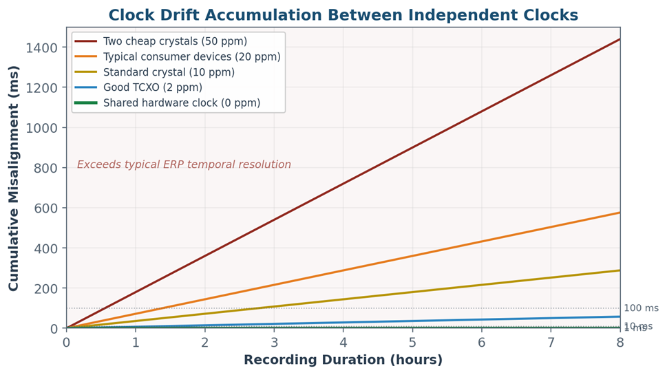
What Drift Looks Like in Practice

These numbers represent cumulative misalignment between two data streams. A 20 ppm relative drift between your eye tracker's clock and your EEG amplifier's clock produces 72 ms of misalignment after just one hour of recording. For any analysis that relies on temporal alignment between these streams (fixation-related potentials, saccade-locked ERPs, gaze-contingent event coding), this drift is a direct source of error that grows throughout the session.

How Each Strategy Handles Drift

TTL Triggers: Immune (But Limited)

TTL event markers are not affected by clock drift because they are discrete hardware events captured by each device's own clock at the moment they arrive. However, TTL triggers only mark events — they do not align continuous data streams. If you need sample-level alignment between two continuous streams (e.g., gaze position and EEG voltage), TTL triggers let you identify corresponding events, but the samples between those events may still drift relative to each other.

USB: No Drift Correction

A USB device's samples are timestamped by the host computer's clock, so there is no inter-device drift within a single machine. However, if you are running devices on separate computers (which is common in multi-device setups), the clocks of those computers will drift independently. USB provides no mechanism to detect or correct this.

Ethernet (Device PC + RTOS): Precise Internally, Drift Between Devices

In the dual-PC approach, gaze data is timestamped by the device PC's own real-time clock, so the gaze samples themselves do not drift relative to each other. The drift problem emerges when aligning this timeline with external devices and the experiment PC. Each PC and device clock is an independent oscillator that will drift apart over time. Event messages and TTL triggers provide periodic anchor points for alignment, but between those anchors, the two clocks accumulate drift. For a typical 1-hour recording with 10–20 ppm relative drift, this could mean 36–72 ms of inter-anchor misalignment — enough to affect analyses like ERP-locked gaze evaluation.

LSL: Active Drift Correction (With Limitations)

LSL's clock synchronization protocol periodically measures the offset between each outlet's clock and the recording machine's clock. These measurements are stored in the XDF file, and importers use them to fit a linear (or piecewise-linear) model of clock drift, which is then applied to correct timestamps post-hoc. This is the most sophisticated software-based approach available, and under good conditions it works well. However, it depends on the assumption that drift is smooth and predictable — sudden changes in temperature, CPU throttling, or power management can cause non-linear drift that the correction model may not capture. It also cannot correct drift faster than the measurement interval (typically a few seconds), leaving sub-second fluctuations uncorrected.

Dedicated Hardware Clock: Drift Eliminated by Design

When all signals share a single hardware clock, there is no drift to correct. It does not matter how long the recording runs — one hour, eight hours, an entire day — the alignment between gaze data, stimulus events, digital triggers, and analog channels remains constant at sub-microsecond precision. This is not because the clock is more accurate in an absolute sense (though FPGA oscillators are typically high-quality), but because there is only one clock. Drift is a multi-clock problem.

Even for external devices like EEG amplifiers that necessarily have their own clocks, the DATAPixx3's architecture helps: the TTL triggers it sends to the amplifier are generated by the FPGA, not by the host computer's OS. This means the trigger anchors themselves are precisely aligned with the stimulus and gaze data. The amplifier's clock still drifts relative to the FPGA clock between anchors, but the anchors are as precise as the hardware can make them.

The solution implemented by Psychtoolbox to correct for clock drift between its own timestamps and the DATAPixx3 clock is fully automated; see the documentation for PsychDataPixx('GetPreciseTime') for details. Psychtoolbox users may also wish to consult documentation for PsychDataPixx('BoxsecsToGetsecs') on the same page to see how clock drift can be modelled and corrected for over time.

When Does Precision Matter?

Not every experiment needs sub-microsecond synchronization. The practical question is: does your analysis method require temporal alignment that exceeds the precision your synchronization strategy provides? Below are common experimental scenarios and the timing tolerance they require.

Designing a Layered Synchronization Architecture

The most robust labs do not rely on a single synchronization method. Instead, they build a layered architecture that matches precision to purpose:

Layer 1: Hardware Clock Backbone

A dedicated timing device like an I/O hub provides the master clock for all critical experimental signals: stimulus onset, participant response timing, neural trigger markers, analog physiological channels, and eye tracking data.

Layer 2: TTL Bridge

TTL triggers connect the hardware clock domain to external devices that cannot be directly integrated (e.g., EEG amplifier, OPM-MEG scanner). The TTL lines are driven by the hardware clock's digital I/O, not by the host computer's OS, ensuring that trigger timing inherits the hardware clock's precision.

Layer 3: Software Convenience Layer

LSL (or equivalent) handles auxiliary and non-critical streams: motion capture, video recording, and any other data where millisecond-scale alignment is sufficient. This layer provides the flexibility and convenience needed for complex multi-device recordings without compromising the timing precision of the core signals.

Conclusion

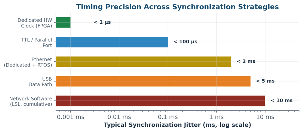
Several strategies exist to solve the fundamental problem of aligning multiple data streams over time. The five strategies described here span six orders of magnitude in timing precision, from sub-microsecond dedicated hardware to multi-millisecond networked software. Each has legitimate use cases, and most labs benefit from combining multiple approaches to balance research needs across complex system integration.

The critical insight is that every synchronization strategy has a quantifiable timing uncertainty budget, and that budget should be evaluated against the temporal demands of your specific analysis before you start collecting data. The worst-case scenario is conducting an entire time-, cost-, and labour-intensive study only to find that the collected data are too temporally imprecise to yield meaningful results. This kind of frustration can be easily avoided by accounting for the system's temporal precision in the experimental design phase.

Software-based synchronization via LSL is a powerful tool for flexible multi-device recording. Ethernet with a real-time OS provides a solid single-device solution. TTL triggers offer nearly universal discrete-event marking across independent systems, but the precision of signal generation matters. For experiments where the science depends on precise temporal alignment between stimulus, gaze, and neural data, dedicated hardware synchronization remains a gold standard for temporal precision.

References

• Kothe, C., et al. (2024/2025). "The Lab Streaming Layer for Synchronized Multimodal Recording." Imaging Neuroscience, MIT Press.

• Brain Products GmbH (2026). "Tips and Tricks for Using Lab Streaming Layer (LSL)."

• ANT Neuro Academy (2025). "Replacing Conventional Parallel Port with USB to TTL Devices."

• SR Research. EyeLink 1000 Plus specifications.

• Psychtoolbox wiki. "FAQ: TTL Triggers via USB."

• LSL FAQ documentation, labstreaminglayer.readthedocs.io.

Questions about synchronization architecture for your lab? Contact VPixx Technologies at support@vpixx.com or visit www.vpixx.com.